Dynamic Characteristic Analysis of Permanent Magnet Brushless DC Motor System with Rolling Rotor

Abstract

With the wide application of permanent magnet brushless DC motors (BLDCMs) in home appliances and electric vehicles, there is increasing demand for BLDCMs with low vibration and noise. This paper aims to study the dynamic characteristics of a type of BLDCM with a rolling rotor. Firstly, a dynamic model of a BLDCM with eighteen degrees of freedom (18 DOFs) is built, for which the electromagnetic force and the oil-film force of the sliding bearing are considered. Then, the system responses are solved by Runge–Kutta numerical method, and the effects of the rotational speed, bearing backlash and eccentric distance of the rolling rotor on the dynamic response are analyzed in detail. The time history, frequency plot, axis trajectory diagram and phase portrait are introduced to discuss the dynamic behavior of the motor system. Analysis results show that eccentric force increases obviously with increasing rotational speed or eccentric distance, which can change the dynamic response through suppressing the electromagnetic force. The effect of bearing clearance on the rotor and stator is negatively correlated. Therefore, system parameters should be determined properly to improve the running performance of the motor system. Numerical results can provide a useful guide for the design and vibration control of such motor systems.

1. Introduction

Permanent magnet BLDCMs have many advantages, such as simple construction, small size, high efficiency and easy control, and they are widely used in many industrial and household fields [1]. In order to improve running performance, this type of motor has been deeply investigated by many researchers, mainly concerning motor design [2,3], electromagnetic analysis [4,5,6], motor control [7,8,9,10], motor detection [11,12] and so on. However, the vibration and noise of BLDCMs become a constraint to their development and are one of the outstanding problems [13].

A review of many published papers concerning vibration and noise suppression of these motors leads to classification of existing methods into three main groups: The first group controls the current, voltage, or speed of the motor [14]. For example, Darba et al. [8] proposed a model-predictive control algorithm to control the speed and current, which improved the dynamic behavior of the BLDCM. Pindoriya et al. [13] used digital pulse-width modulation for speed control to analyze the vibration and noise of a BLDCM under different operating points. Muhammed et al. [15] used artificial intelligence to estimate rotor speed of a BLDCM, in which the predicted results have high accuracy. Based on field-oriented control, Hao et al. [16] proposed a novel control strategy to produce an artificially pulsating torque and thus reduce the radial vibration of the permanent magnet motor. This method focuses on the study of new algorithms or prediction models to better control the motor.

The second group investigates the electromagnetic field of the motor and further analyzes the effect of electric magnetization on system dynamics. For example, Huang et al. [17] evaluated the exciting force of a permanent magnet motor to optimize the motor parameters, including stator winding, rotor permanent magnet shape and skew angle. Considering the dynamic and static eccentricity, Guo et al. [18] calculated the unbalanced magnetic pull (UMP) to investigate its effect on the vibration response of the motor. Zhu et al. [19] analyzed the radial vibration force by finite element method and studied the influence of stator slotting and air gap on the vibration force. By alternating the distribution of the radial flux density, Hur et al. [20] carried out harmonic elimination of vibration and noise of a permanent magnet motor. Ma et al. [21] presented a new method to calculate electromagnetic torque in a permanent magnet synchronous motor and studied the effect of sixth-order torque ripple on the vibration and noise of electric vehicles.

From the structural dynamics point of view, another method emphatically analyzes the dynamic characteristics of the motor system to optimize structural parameters, achieving the reduction of the vibration and noise. Mohammed et al. [22] presented a state-space technique to analyze the dynamic performance of permanent magnet BLDCMs. Considering the air gap variation between the rotor and the stator, Im et al. [23] built a dynamic model of a BLDCM in which the displacements and currents were coupled, and researched the dynamic behavior of the system. Based on the built dynamic model [23], Im et al. [24] further designed a new BLDCM with higher torque, higher speed and lower vibration. Considering the effect of unbalanced magnetic pull, Zhang et al. [25] established the dynamic model of an offset rotor-bearing system for a permanent magnet synchronous motor and investigated the dynamic characteristics under varying parameters, including rotor offsets, radial clearances and static displacement eccentricities. Based on a mathematical model of a permanent magnet BLDC in-wheel motor system, Li et al. [26] investigated the electromechanical coupling vibration of the system caused by the distortion of the air gap magnetic field. Although the dynamic characteristics of BLDCMs has been reported, the dynamics of BLDCMs with rolling rotors have received very little attention. Thus, the main goal of this paper is to investigate the dynamic characteristics of a BLDCM with a rolling rotor considering electromagnetic and bearing forces.

The remainder of this paper is organized as follows. In Section 2, a dynamic model of a BLDCM with 18 DOFs is established, considering the effect of the oil-film force of the sliding bearing and the electromagnetic force. In Section 3, the dynamic characteristics of the BLDCM are analyzed to quantify the effect of the parameters on the dynamic response. Finally, some conclusions are revealed in Section 4.

2. Dynamic Model of the Rotor–Bearing–Stator System for the BLDCM

2.1. Model of the BLDCM

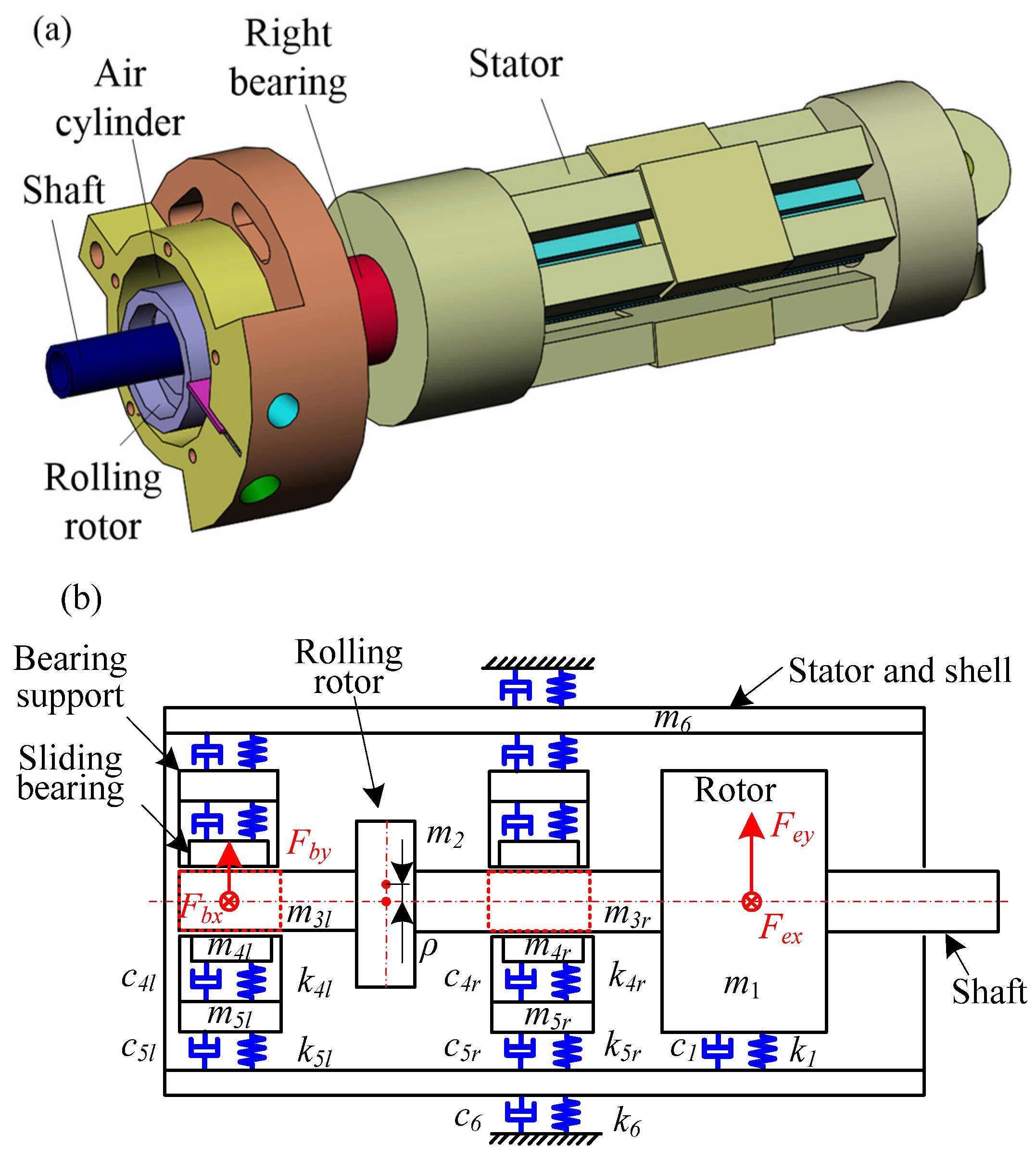
A BLDCM mainly consists of the rotor, stator, rolling rotor, shaft, sliding bearing and shell, as shown in Figure 1a. To research the dynamic characteristics of the BLDCM, a simplified lumped parameter model is built, as shown in Figure 1b, where the uncertain factors [27] are neglected.

In Figure 1b, the bearings and supports are described as springs and damping. The symbols k₁ and c₁ are the lateral stiffness and damping of the rotor, respectively; k₂ and c₂ are the lateral stiffness and damping of the rolling rotor, respectively; k_il and c_i1 (i = 4, 5) represent the lateral stiffness and damping of the left sliding bearing and its support, respectively. Similarly, the right bearing and support have the relative parameters, including k_ir and c_ir (i = 4, 5); k₆ and c₆ are the support stiffness and damping of the shell; m₁, m₂ and m₆ are masses of the rotor, rolling rotor and shell, respectively; m_3l, m_4l and m_5l are the masses of the left shaft neck, the sliding bearing and the support, respectively; F_ex and F_ey are the electromagnetic force and torque acting on the rotor along the x and y directions, respectively; F_bx and F_by are the oil-film forces along x and y directions, respectively. In addition, ρ is the eccentric distance of the rolling rotor.

2.2. Oil-Film Force of Sliding Bearing

Considering the change of oil-film thickness, the Reynolds equation can be described as

$$\frac{1}{R_r^2}\frac{\partial }{\partial \theta }\left(\frac{h^3}{12\eta }\frac{\partial p}{\partial \theta }\right)=\frac{1}{2}(\omega -2{\dot{\psi }}_r)\frac{\partial h}{\partial \theta }+{\dot{e}}_r\cos \theta$$

(1)

$$h=C(1+\epsilon cos\theta )$$

(2)

where R_r is the radius of the shaft neck, h is the oil-film thickness, η is lubricating oil viscosity, P is the oil-film pressure, ω is rotational speed, e_r is the eccentric distance of the shaft neck, ψ is the angle between the center of the shaft neck and the horizontal direction, ε is the eccentricity ratio of the shaft neck, and C is the bearing radius clearance.

The oil-film forces of the right sliding bearing along the radial and tangential directions can be derived as

$$\begin{array}{l}{F}_{rr}=6\eta R_r{L}_r{(\frac{R}{C})}^2\left[(\omega -2{\dot{\psi }}_r)E_1(e_r)+2\dot{\epsilon }{E}_2(e_r)\right]\\ F_{tr}=6\eta R_r{L}_r{(\frac{R}{C})}^2\left[(\omega -2{\dot{\psi }}_r)E_3(e_r)+2\dot{\epsilon }{E}_4(e_r)\right]\end{array}$$

(3)

where

$$\begin{array}{l}{E}_1(e_r)=\frac{2{\epsilon }^2}{(1-{\epsilon }^2)(2+{\epsilon }^2)}\\ E_2(e_r)=\frac{1}{{(1-{\epsilon }^2)}^{3/2}}\left[\frac{\pi }{2}-\frac{8}{\pi (2+{\epsilon }^2)}\right]\\ E_3(e_r)=\frac{\pi \epsilon }{{(1-{\epsilon }^2)}^{1/2}(2+{\epsilon }^2)}\\ E_4(e_r)=\frac{2\epsilon }{(1-{\epsilon }^2)(2+{\epsilon }^2)}\end{array}$$

(4)

Thus, the oil-film forces between the right sliding bearing and shaft along the horizontal and vertical directions can be expressed by

$$\begin{array}{l}{F}_{xr}=F_{rr}\sin {\psi }_r-F_{tr}\cos {\psi }_r\\ F_{yr}=-F_{rr}cos{\psi }_r-F_{tr}\sin {\psi }_r\end{array}$$

(5)

Similarly, the left oil-film forces can be described as

$$\begin{array}{l}{F}_{xl}=F_{rl}\sin {\psi }_l-F_{tl}\cos {\psi }_l\\ F_{yl}=-F_{rl}cos{\psi }_l-F_{tl}\sin {\psi }_l\end{array}$$

(6)

2.3. Electric Magnetization Analysis of the BLDCM

Based on the relationship between the magnetic flux density and the magnetic vector potential, the radial and tangential magnetic flux density in the air gap can be obtained by

$$\begin{array}{l}{B}_r={\displaystyle \sum _{n=1}^{\infty }\left[P_{1n}sin(n\phi )+P_{3n}cos(n\phi )\right]}\\ B_{\phi }={\displaystyle \sum _{n=1}^{\infty }\left[P_{2n}sin(n\phi )+P_{4n}cos(n\phi )\right]}\end{array}$$

(7)

where

$$\begin{array}{l}{P}_{1n}=-\frac{1}{r}[E_n{R}_1\frac{S_n(r,R_2)}{T_n(R_1,R_2)}+F_n{R}_2\frac{S_n(r,R_1)}{T_n(R_2,R_1)}]\\ P_{2n}=-\frac{1}{r}[G_n{R}_1\frac{T_n(r,R_2)}{T_n(R_1,R_2)}+H_n{R}_2\frac{T_n(r,R_1)}{T_n(R_2,R_1)}]\\ P_{3n}=\frac{1}{r}[G_n{R}_1\frac{S_n(r,R_2)}{T_n(R_1,R_2)}+H_n{R}_2\frac{S_n(r,R_1)}{T_n(R_2,R_1)}]\\ P_{4n}=-\frac{1}{r}[E_n{R}_1\frac{T_n(r,R_2)}{T_n(R_1,R_2)}+F_n{R}_2\frac{T_n(r,R_1)}{T_n(R_2,R_1)}]\end{array}$$

(8)

where n is a positive integer, R₁ and R₂ are inside and outside radii, respectively, E_n, F_n, G_n and H_n refer to the harmonic coefficients of the magnetic vector potential in the air gap, and functions S and T are used to deal with the solutions of the magnetic vector potential.

The electromagnetic torque can be expressed by

$$T_e=\frac{L_m{r}^2}{{\mu }_0}{\displaystyle {\int }_0^{2\pi }{B}_r(r,\phi )}{B}_{\phi }(r,\phi )d\phi \hspace{1em}\hspace{1em}{R}_1<r<R_2$$

(9)

where L_m is the axial length of the stator core, and μ₀ is the air gap permeability.

Substituting Equation (7) into Equation (9), the electromagnetic torque can be described by the Fourier series

$$T_e=\frac{\pi L_m{r}^2}{{\mu }_0}{\displaystyle \sum _{n=1}^{\infty }(P_{1n}{P}_{2n}{P}_{3n}{P}_{4n})}$$

(10)

Based on the Maxwell tensor formula, the electromagnetic forces along the x and y directions can be written as

$$\begin{array}{l}{F}_{ex}=\frac{L_{m}r}{2{\mu }_0}{\displaystyle {\int }_0^{2\pi }[(B_r^2-B_{\phi }^2)cos\phi -2B_r{B}_{\phi }sin\phi ]}d\phi \\ F_{ey}=\frac{L_{m}r}{2{\mu }_0}{\displaystyle {\int }_0^{2\pi }[(B_r^2-B_{\phi }^2)sin\phi +2B_r{B}_{\phi }cos\phi ]}d\phi \end{array}$$

(11)

Then, substituting the magnetic flux densities of Equation (7) into Equations (10) and (11) results in:

$$\begin{array}{l}{F}_{ex}=\frac{\pi L_{m}r}{4{\mu }_0}{\displaystyle \sum _{\left|j-n\right|=1}(P_{1j}{P}_{1n}-P_{2j}{P}_{2n}+P_{3j}{P}_{3n}-P_{4j}{P}_{4n})}\\ \hspace{1em}\hspace{1em} -\frac{\pi L_{m}r}{2{\mu }_0}[{\displaystyle \sum _{j-n=1}(P_{1j}{P}_{2n}-P_{3j}{P}_{4n})-{\displaystyle \sum _{j-n=-1}(P_{1j}{P}_{2n}-P_{3j}{P}_{4n})}}]\\ F_{ey}=\frac{\pi L_{m}r}{4{\mu }_0}{\displaystyle \sum _{j-n=1}(P_{1j}{P}_{3n}-P_{3j}{P}_{1n}-P_{2j}{P}_{4n}+P_{4j}{P}_{2n})}\\ \hspace{1em}\hspace{1em} -\frac{\pi L_{m}r}{4{\mu }_0}{\displaystyle \sum _{j-n=-1}(P_{1j}{P}_{3n}-P_{3j}{P}_{1n}-P_{2j}{P}_{4n}+P_{4j}{P}_{2n})}\\ \hspace{1em}\hspace{1em} +\frac{\pi L_{m}r}{2{\mu }_0}{\displaystyle \sum _{\left|j-n\right|=1}(P_{1j}{P}_{2n}+P_{3j}{P}_{4n})}\end{array}$$

(12)

2.4. Equations of Motion

Figure 1 demonstrates the simplified generalized lumped dynamic model of the BLDCM system. The system has eighteen lateral degrees of freedom (DOF), including two laterals of the rotor (x₁ and y₁), two laterals of the rolling rotor (x₂ and y₂), two laterals of the left shaft neck, sliding bearing and support, respectively (x_3l, y_3l, x_4l, y_4l, x_5l and y_5l), two laterals of the right shaft neck, sliding bearing and support, respectively (x_3r, y_3r, x_4r, y_4r, x_5r and y_5r), and two laterals of the shell (x₆ and y₆), ignoring the torsional and axial DOFs. Thus, the corresponding coordinate vector of the motor system can be described by

$$\begin{array}{l}X=[\begin{array}{ccccccccc}{x}_1& y_1& x_2& y_2& x_{3r}& y_{3r}& x_{3l}& y_{3l}& x_{4r}\end{array}\\ \hspace{1em}\hspace{1em}\begin{array}{ccccccccc}{y}_{4r}& x_{4l}& y_{4l}& x_{5r}& y_{5r}& x_5{}_l& y_{5l}& x_6& y_6\end{array}{]}^T\end{array}$$

(13)

The kinetic energy T, potential energy U, and dissipation function R of the BLDCM system are represented as the following expressions:

$$\begin{array}{l}T=\frac{1}{2}[m_1({\dot{x}}_1^2+{\dot{y}}_1^2)+m_2({\dot{x}}_2^2+{\dot{y}}_2^2)+m_{3r}({\dot{x}}_{3r}^2+{\dot{y}}_{3r}^2)+\\ \hspace{1em}\hspace{1em}\hspace{1em}{m}_{3l}({\dot{x}}_{3l}^2+{\dot{y}}_{3l}^2)+m_{4r}({\dot{x}}_{4r}^2+{\dot{y}}_{4r}^2)+m_{4l}({\dot{x}}_{4l}^2+{\dot{y}}_{4l}^2)+\\ \hspace{1em}\hspace{1em}\hspace{1em}{m}_{5r}({\dot{x}}_{5r}^2+{\dot{y}}_{5r}^2)+m_{5l}({\dot{x}}_{5l}^2+{\dot{y}}_{5l}^2)+m_6({\dot{x}}_6^2+{\dot{y}}_6^2)]\end{array}$$

(14)

$$\begin{array}{l}U=\frac{1}{2}[k_1{(x_1-x_{3r})}^2+k_1{(y_1-y_{3r})}^2+k_2{(x_2-x_{3r})}^2+k_2{(y_2-y_{3r})}^2+\\ \hspace{1em}\hspace{1em}\hspace{1em}{k}_2{(x_2-x_{3l})}^2+k_2{(y_2-y_{3l})}^2+k_{4r}{(x_{4r}-x_{5r})}^2+k_{4r}{(y_{4r}-y_{5r})}^2+\\ \hspace{1em}\hspace{1em}\hspace{1em}{k}_{4l}{(x_{4l}-x_{5l})}^2+k_{4l}{(y_{4l}-y_{5l})}^2+k_{5r}{(x_{5r}-x_6)}^2+k_{5r}{(y_{5r}-y_6)}^2+\\ \hspace{1em}\hspace{1em}\hspace{1em}{k}_{5l}{(x_{5l}-x_6)}^2+k_{5l}{(y_{5l}-y_6)}^2+k_2(x_6^2+y_6^2)]\end{array}$$

(15)

$$\begin{array}{l}R=\frac{1}{2}[c_1{({\dot{x}}_1-{\dot{x}}_{3r})}^2+c_1{({\dot{y}}_1-{\dot{y}}_{3r})}^2+c_2{({\dot{x}}_2-{\dot{x}}_{3r})}^2+c_2{({\dot{y}}_2-{\dot{y}}_{3r})}^2+\\ \hspace{1em}\hspace{1em}\hspace{1em}{c}_2{({\dot{x}}_2-{\dot{x}}_{3l})}^2+c_2{({\dot{y}}_2-{\dot{y}}_{3l})}^2+c_{4r}{({\dot{x}}_{4r}-{\dot{x}}_{5r})}^2+c_{4r}{({\dot{y}}_{4r}-{\dot{y}}_{5r})}^2+\\ \hspace{1em}\hspace{1em}\hspace{1em}{c}_{4l}{({\dot{x}}_{4l}-{\dot{x}}_{5l})}^2+c_{4l}{({\dot{y}}_{4l}-{\dot{y}}_{5l})}^2+c_{5r}{({\dot{x}}_{5r}-{\dot{x}}_6)}^2+c_{5r}{({\dot{y}}_{5r}-{\dot{y}}_6)}^2+\\ \hspace{1em}\hspace{1em}\hspace{1em}{c}_{5l}{({\dot{x}}_{5l}-{\dot{x}}_6)}^2+c_{5l}{({\dot{y}}_{5l}-{\dot{y}}_6)}^2+c_2({\dot{x}}_6^2+{\dot{y}}_6^2)]\end{array}$$

(16)

The force vector F of the BLDCM system can be expressed as follows:

$$\begin{array}{l}F=diag[F_{ex}{F}_{ey}-m_{1}g{m}_2\rho {\omega }^2\cos (\omega t)m_2\rho {\omega }^{2}sin(\omega t)-m_{2}g\\ \hspace{1em}\hspace{1em}\hspace{1em}\hspace{1em}{F}_{rx}{F}_{ry}-m_{3r}g{F}_{lx}{F}_{ly}-m_{3l}g-F_{rx}-F_{ry}-m_{4l}g\\ \hspace{1em}\hspace{1em}\hspace{1em}\hspace{1em}-F_{lx}-F_{ly}-m_{4l}g0000-F_{ex}-F_{ey}-m_{6}g{]}^T\end{array}$$

(17)

The differential equations of the motor system can be derived by Lagrange’s equation as follows:

$$\frac{\partial }{\partial t}\left(\frac{\partial T}{\partial \dot{X}}\right)-\frac{\partial T}{\partial X}+\frac{\partial U}{\partial X}+\frac{\partial R}{\partial \dot{X}}=F$$

(18)

Substituting Equations (13)–(17) into Equation (18), the differential equations of the motor system can be written in the form of matrix:

$$M\ddot{X}+C\dot{X}+KX=F$$

(19)

where M, C and K are the mass matrix, damping matrix and stiffness matrix, respectively, which are shown in Appendix A.

3. Dynamic Response of the BLDCM System

A BLDCM is a complex dynamic system due to the existence of bearing backlash, eccentric distance, excitation current, manufacturing and installation errors and so on. In order to improve the running performance of the motor system, it is essential to optimize the structural parameters by investigating the system dynamic characteristics comprehensively. The rotational speed Ω, bearing backlash b, and the eccentric distance of the rolling rotor ρ are selected as the control parameters to analyze their effects on the dynamic responses of the system through the ode45 Runge–Kutta method, where the initial conditions are $\mathrm{X}\left(0\right)=0$ and $\dot{\mathrm{X}}\left(0\right)=0$. The dynamic behaviors of the motor system are identified and discussed from the time history, the frequency plot, the axis trajectory diagram and the phase portrait. The concerned system parameters are listed in

Table 1. Parameters of the BLDCM system.

Parameters	Value
Rated power (kw)	1.5
Mass of rotor m1 (kg)	0.84
Mass of rolling rotor m2 (kg)	0.23
Mass of left shaft neck m3l (kg)	0.05
Mass of left sliding bearing m4l (kg)	0.19
Mass of left support m5l (kg)	0.89
Mass of shell m6 (kg)	5.33
Stiffness k1, 2 (N/m)	3.07 × 105
Stiffness k4r, 4l (N/m)	1.7 × 105
Stiffness k5r, 5l (N/m)	3.6 × 105
Stiffness k6 (N/m)	2.8 × 105
Damping c1, 2 (N/(m·s))	800
Damping c4r, 4l (N/(m·s))	660
Damping c5r, 5l (N/(m·s))	540
Damping c6 (N/(m·s))	600

.

3.1. Analysis of the Effects of Rotational Speed

For a motor system, rotational speed Ω is one of the key physical parameters. Thus, this subsection mainly studies the effect of rotational speed on the dynamic response of the motor system, in which the vibration responses of the rotor and stator are taken for example. During normal operation conditions, the rotational speed of the motor system is in the range of 1200 r/min < Ω < 9000 r/min, i.e., 20 rps < Ω < 150 rps.

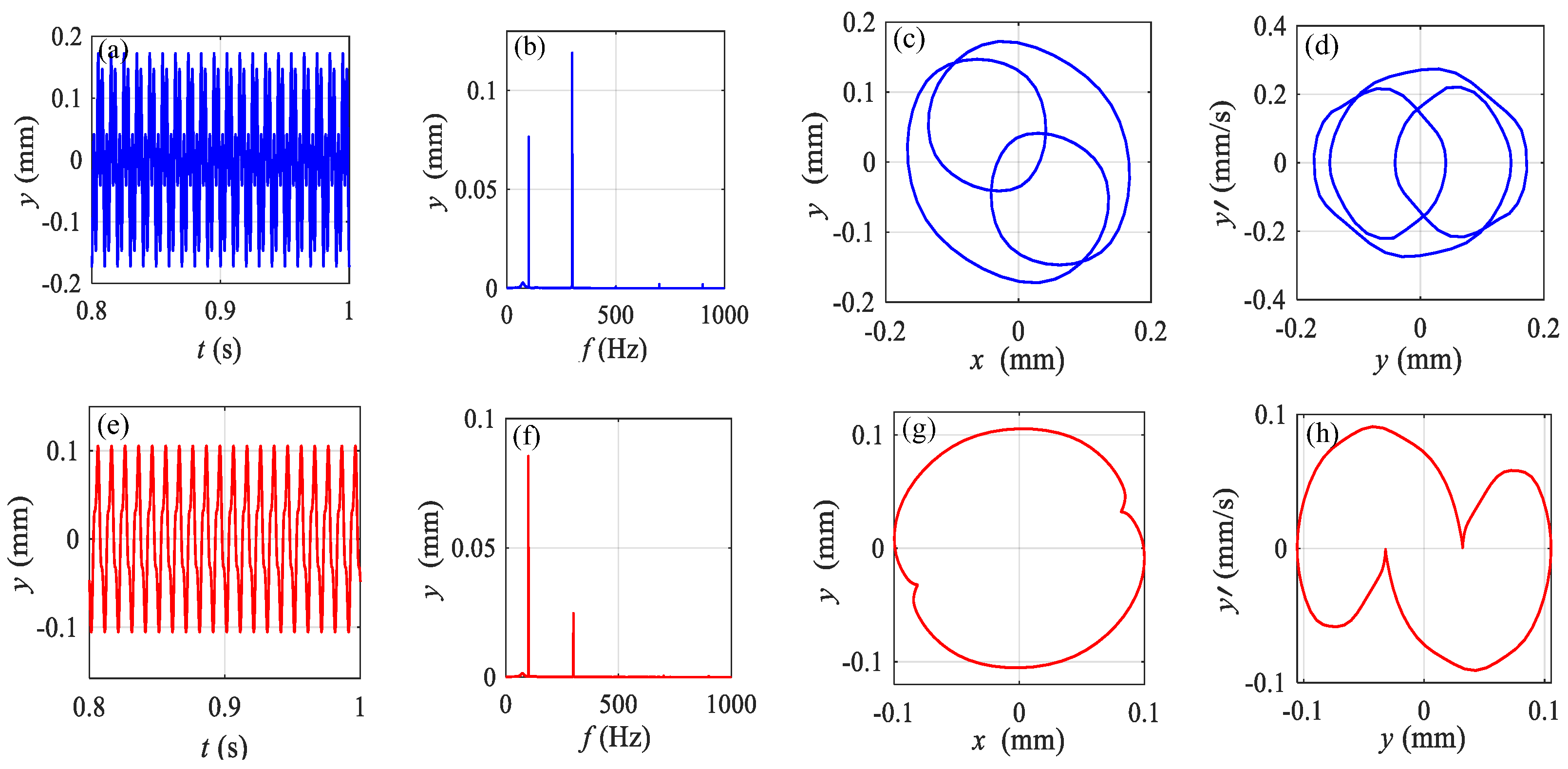
Other system parameters remain unchanged and mainly include the bearing backlash b = 5 × 10⁻⁵ m and the eccentric distance of the rolling rotor ρ = 1 × 10⁻³ m. Under three different rotational speeds, namely Ω = 100 rps, 120 rps and 150 rps, the corresponding vibration responses along the y direction are shown in Figure 2, Figure 3 and Figure 4, where subfigures a–d and subfigures e–h indicate the dynamic features of the rotor and stator, respectively. At Ω = 100 rps, the rotor presents multi-period motion, which can be seen in Figure 2a,d. The frequency spectrum shows two main harmonic components in Figure 2b, i.e., the rotational frequency (f_r = 100 Hz) and the multiplication frequency (3f_r = 300 Hz). This is due to the eccentricity of the rolling rotor and the electromagnetic force. The response amplitude at 3f_r dominates, the amplitude at f_r is second largest, and the amplitude at other frequencies is negligible. The axis trajectory diagram in Figure 2c shows a complicated closed non-circular curve, which is caused by the combined action of the eccentric force and electromagnetic force. When Ω increases to 120 rps, the vibration amplitude of the rotor reduces obviously in Figure 3a. However, the components of the frequency spectrum in Figure 3b are unchanged, where 3f_r (360 Hz) is still dominant. Compared to the axis trajectory diagram in Figure 2c, the range of the axis trajectory diagram in Figure 3c decreases. Although the motion state in Figure 3d is similar to that in Figure 2d, the system under Ω = 120 rps shows smaller vibration response. However, when Ω further increases to 150 rps, the rotational frequency (f_r = 150 Hz) in Figure 4b becomes the main response since the eccentric force increases. The corresponding axis trajectory diagram also shows a simpler curve in Figure 4c. This reveals that there is a better rotational speed to make the motor system more stable.

For the stator, under different rotational speeds, its dynamic responses are always smaller compared with those of the rotor, such as Figure 2a,e. Furthermore, the rotational frequency usually occupies the main component, which can be seen in Figure 2f, Figure 3f and Figure 4f. Meantime, the corresponding axis trajectory diagrams are simple compared with those of the rotor. The response results reveal that the electromagnetic force leads to the complex dynamic features of the motor, which should be further investigated in the future.

In order to visually demonstrate the influence of rotational speed on the motor system, the 3D dynamic response curves under different speeds are shown in Appendix B, which assists in the description of the response results.

3.2. Analysis of the Effects of the Eccentric Distance

To investigate the effect of the eccentric distance of the rolling rotor on the dynamic characteristic of the motor system, the eccentric distance ρ is chosen as the control parameter. The other system parameters are set as follows: rotational speed Ω = 100 rps, and bearing backlash b = 5 × 10⁻⁵ m. Then, the dynamic behaviors of the rotor and stator with ρ = 3 × 10⁻³ m and 5 × 10⁻³ m are illustrated in Figure 5 and Figure 6, respectively.

Comparing Figure 2a, Figure 5a and Figure 6a, it can be clearly seen that the vibration amplitude gradually increases with the increase in the eccentric distance. However, under the three eccentric distances, the motor system is always multiple periodic. This signifies that the increasing eccentric force deteriorates the dynamic characteristic of the motor system, which becomes the main source of system vibration. The frequency plot verifies this finding. In Figure 2b, 3f_r is the main response, whereas the rotational frequency f_r in Figure 5b and Figure 6b occupies the main component. The increasing eccentric force also leads to simplification of the axis trajectory diagram of the rotor, but the corresponding trajectory ranges increase, which can be seen in Figure 2c, Figure 5c and Figure 6c. This phenomenon also appears in the stator. When the eccentric distance increases, the axis trajectory diagram of the stator gradually becomes a circular curve, as shown in Figure 2g, Figure 5g and Figure 6g. Therefore, the eccentric distance should be reduced as far as possible in the design processing of the rolling rotor, such as by increasing the balance block or reducing the amount of material on the eccentric side.

Similarly, under different eccentric distances, the corresponding 3D dynamic response curves are shown in Appendix B.

3.3. Analysis of the Effects of the Bearing Clearance

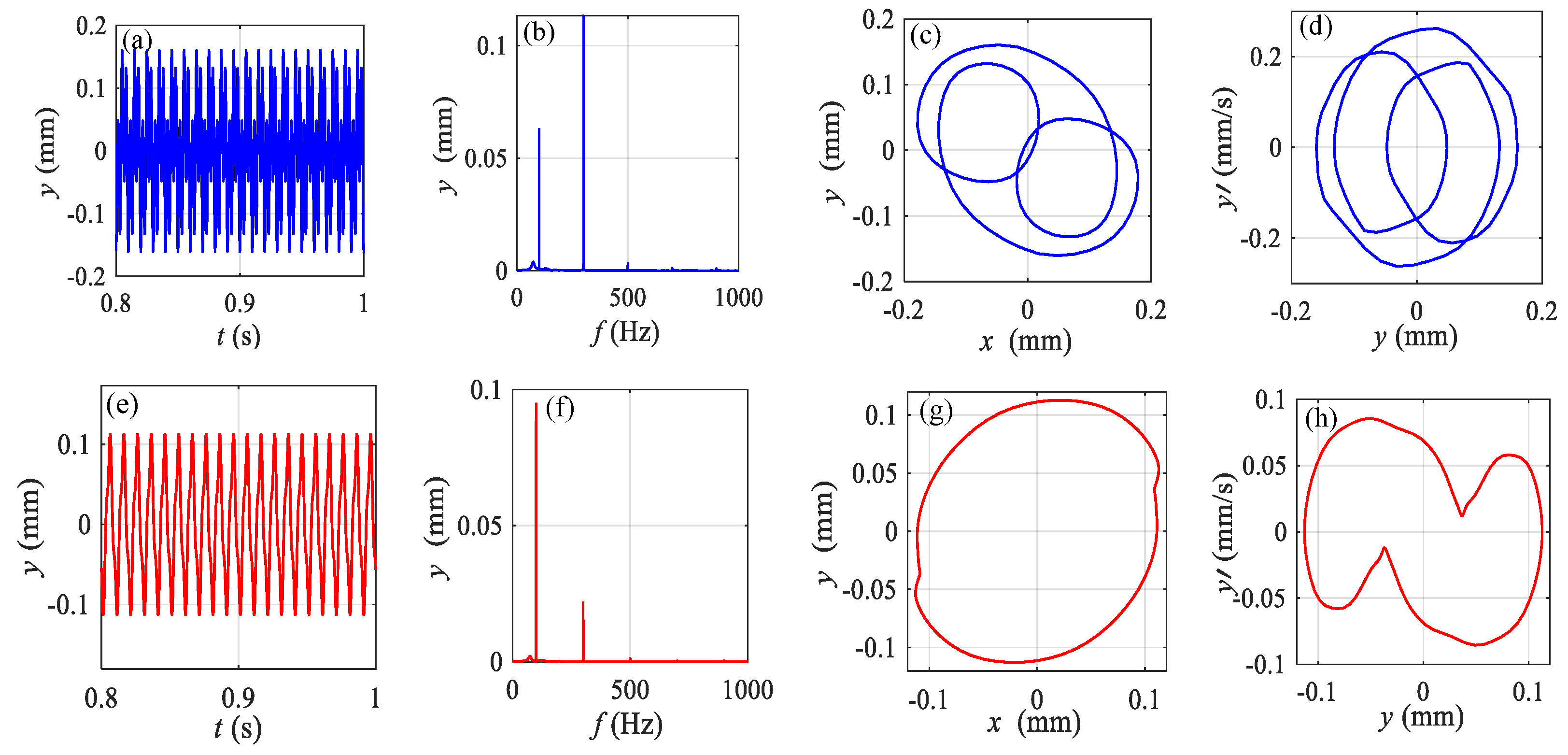
In rotating equipment, backlash, such as gear backlash and bearing clearance, easily leads to complex dynamic behaviors of the system [28,29]. Therefore, it is vital to analyze the effect of bearing clearance on motor systems. As the control parameter, three bearing clearances, b = 3 × 10⁻⁵ m, 8 × 10⁻⁵ m and 12 × 10⁻⁵ m, are chosen. The other system parameters are as follows: rotational speed Ω = 100 rps, and eccentric distance of the rolling rotor ρ = 1 × 10⁻³ m. The corresponding dynamic responses are shown in Figure 7, Figure 8 and Figure 9. Meanwhile, Figure 2 presents the vibration response when b = 5 × 10⁻⁵ m.

When the bearing clearance increases from 3 × 10⁻⁵ m to 12 × 10⁻⁵ m, the spectral components of the rotor and stator are unchanged in the frequency spectrums of Figure 2b,f, Figure 7b,f, Figure 8b,f and Figure 9b,f. For example, the multiplication frequency (3f_r) in the frequency plot of the rotor is the main response, and the rotational frequency (f_r) of the stator is the dominant response. The numerical results indicate that varying bearing clearance has no effect on the eccentric force and electromagnetic force. However, when the bearing clearance increases, the amplitudes of the vibration response of the rotor decrease gradually, and those of the stator increase. Specifically, the corresponding response amplitudes of the rotor are 0.126 mm, 0.122 mm, 0.119 mm and 0.113 mm, and those of the stator are 0.076 mm, 0.078 mm, 0.085 mm and 0.095 mm, respectively. Similarly, as the bearing clearance increases, the axis trajectory diagrams of the rotor become smaller, whereas the trajectory ranges of the stator gradually increase. According to the above analysis, to keep the better running performance of the rotor and the stator simultaneously, the bearing clearance should be selected properly.

In addition, with different bearing clearances, the relative 3D dynamic response curves are shown in Appendix B.

4. Conclusions

We build an 18-DOF lateral dynamic model of a BLDCM system and preliminarily investigate the effects of structural parameters on the dynamic characteristic of the system. The analysis results not only provide better understanding of the dynamic characteristics of the BLDCM system, but also present a useful source of reference to improve the running performance of motor systems through optimizing the important parameters.

Numerical results reveal that increasing rotational speed and eccentric distance can the enhance eccentric force and further suppress the electromagnetic force, which will change the dynamic behavior of the motor system. When the bearing clearance increases, the dynamic response of the motor can be improved, whereas that of the stator will be deteriorated. Overall, the proper values of system parameters, such as the rotational speed, eccentric distance, and bearing clearance, should be chosen to reduce vibration amplitude to improve the running performance of the motor system.

Though the dynamic features of a motor system are studied in this paper, there exist some important topics that should be further investigated in the future. The dynamic model of the motor system should be improved, such as the lateral–torsional–axial-coupled dynamic model. More factors should be considered, such as the external excitation, the rub–impact force, sources of uncertainty and so on. In addition, vibration testing of the motor will also be required to verify the accuracy of the numerical analysis.

References

- Cheng, M.; Hua, W.; Zhang, J.; Zhao, W. Overview of Stator-Permanent Magnet Brushless Machines. IEEE Trans. Ind. Electron. 2011, 58, 5087–5101. [Google Scholar] [CrossRef]
- Amor, M.B.; Tounsi, S.; Bouhlel, M.S. Design and Optimization of Axial Flux Brushless DC Motor Dedicated to Electric Traction. Am. J. Electr. Power Energy Syst. 2015, 4, 42. [Google Scholar] [CrossRef] [Green Version]
- Patel, A.N.; Suthar, B.N. Design Optimization of Axial Flux Surface Mounted Permanent Magnet Brushless DC Motor for Electrical Vehicle Based on Genetic Algorithm. Int. J. Eng. 2018, 31, 1050–1056. [Google Scholar]
- Mi, C.; Filippa, M.; Liu, W.; Ma, R. Analytical Method for Predicting the Air-Gap Flux of Interior-Type Permanent-Magnet Machines. IEEE Trans. Magn. 2004, 40, 50–58. [Google Scholar] [CrossRef]
- Dubas, F.; Espanet, C. Analytical Solution of the Magnetic Field in Permanent-Magnet Motors Taking into Account Slotting Effect: No-Load Vector Potential and Flux Density Calculation. IEEE Trans. Magn. 2009, 45, 2097–2109. [Google Scholar] [CrossRef]
- Lubin, T. Two-Dimensional Analytical Calculation of Magnetic Field and Electromagnetic Torque for Surface-Inset Permanent-Magnet Motors. IEEE Trans. Magn. 2012, 48, 2080–2091. [Google Scholar] [CrossRef]
- Olejnik, P.; Adamski, P.; Batory, D.; Awrejcewicz, J. Adaptive Tracking PID and FOPID Speed Control of an Elastically Attached Load Driven by a DC Motor at Almost Step Disturbance of Loading Torque and Parametric Excitation. Appl. Sci. 2021, 11, 679. [Google Scholar] [CrossRef]
- Darba, A.; Belie, F.D.; D’Haese, P.; Melkebeek, J.A. Improved Dynamic Behavior in BLDC Drives Using Model Predictive Speed and Current Control. IEEE Trans. Ind. Electron. 2016, 63, 728–740. [Google Scholar] [CrossRef]
- Santra, S.B.; Chatterjee, A.; Chatterjee, D.; Padmanaban, S.; Bhattacharya, K. High Efficiency Operation of Brushless DC Motor Drive Using Optimized Harmonic Minimization Based Switching Technique. IEEE Trans. Ind. Appl. 2022, 58, 2122–2133. [Google Scholar] [CrossRef]
- Ha, D.H.; Kim, R. Nonlinear Optimal Position Control with Observer for Position Tracking of Surfaced Mounded Permanent Magnet Synchronous Motors. Appl. Sci. 2021, 11, 10992. [Google Scholar] [CrossRef]
- Park, J.K.; Hur, J. Detection of Inter-Turn and Dynamic Eccentricity Faults Using Stator Current Frequency Pattern in IPM-Type BLDC Motors. IEEE Trans. Ind. Electron. 2016, 63, 1771–1780. [Google Scholar] [CrossRef]
- Shifat, T.A.; Hur, J.W. EEMD Assisted Supervised Learning for the Fault Diagnosis of BLDC Motor Using Vibration Signal. J. Mech. Sci. Technol. 2020, 34, 3981–3990. [Google Scholar] [CrossRef]
- Pindoriya, R.M.; Mishra, A.K.; Rajpurohit, B.S.; Kumar, R. An Analysis of Vibration and Acoustic Noise of BLDC Motor Drive. In Proceedings of the 2018 IEEE Power & Energy Society General Meeting (PESGM), Portland, OR, USA, 5–10 August 2018. [Google Scholar]
- Nakata, K.; Hiramoto, K.; Sanada, M.; Morimoto, S.; Takeda, Y. Noise Reduction for Switched Reluctance Motor with a Hole. In Proceedings of the Power Conversion Conference, Osaka, Japan, 2–5 April 2002. [Google Scholar]
- Unlersen, M.F.; Balci, S.; Aslan, M.F.; Sabanci, K. The Speed Estimation via BiLSTM-Based Network of a BLDC Motor Drive for Fan Applications. Arab. J. Sci. Eng. 2022, 47, 2639–2648. [Google Scholar] [CrossRef]
- Hao, Z.; Zhao, R.X.; Zhu, M.L.; Omori, H.; Gamo, K. A Novel Control Strategy for Vibration Reduction in the Permanent Magnet Motor Drive System with Eccentric Load. In Proceedings of the International Conference on Electrical Machines and Systems (ICEMS), Tokyo, Japan, 15–18 November 2009. [Google Scholar]
- Huang, S.; Aydin, M.; Lipo, T.A. Electromagnetic Vibration and Noise Assessment for Surface Mounted PM Machines. In Proceedings of the Power Engineering Society Summer Meeting, Vancouver, BC, Canada, 15–19 July 2001. [Google Scholar]
- Guo, D.; Chu, F.; Chen, D. The Unbalanced Magnetic Pull and Its Effects on Vibration in a Three-phase Generator with Eccentric Rotor. J. Sound Vib. 2002, 254, 297–312. [Google Scholar] [CrossRef]
- Zhu, Z.; Xia, Z.; Wu, L.; Jewell, G.W. Analytical Modeling and Finite-Element Computation of Radial Vibration Force in Fractional-Slot Permanent-Magnet Brushless Machines. IEEE Trans. Ind. Appl. 2010, 46, 1908–1918. [Google Scholar] [CrossRef]
- Hur, J.; Reu, J.; Kim, B.; Kang, G. Vibration Reduction of IPM-Type BLDC Motor Using Negative Third Harmonic Elimination Method of Air-Gap Flux Density. IEEE Trans. Ind. Appl. 2011, 47, 1300–1309. [Google Scholar]
- Ma, C.; Zuo, S.; He, L.; Meng, S.; Sun, Q. Analytical Calculation of Electromagnetic Torque in Permanent Magnet Synchronous Motor for Electric Vehicles. J. Vib. Meas. Diagn. 2012, 32, 756–761. [Google Scholar]
- Mohammed, J. Modeling and Dynamic Performance Analysis of PMBLDC Motor. Eng. Technol. J. 2010, 28, 6091–6107. [Google Scholar]
- Im, H.; Hong, H.; Chung, J. Dynamic Analysis of a BLDC Motor with Mechanical and Electromagnetic Interaction due to Air Gap Variation. J. Sound Vib. 2011, 330, 1680–1691. [Google Scholar] [CrossRef]
- Im, H.; Bae, D.S.; Chung, J. Design Sensitivity Analysis of Dynamic Responses for a BLDC Motor with Mechanical and Electromagnetic Interactions. J. Sound Vib. 2012, 331, 2070–2079. [Google Scholar] [CrossRef]
- Zhang, A.; Bai, Y.; Yang, B.; Li, H. Analysis of Nonlinear Vibration in Permanent Magnet Synchronous Motors under Unbalanced Magnetic Pull. Appl. Sci. 2018, 8, 113. [Google Scholar] [CrossRef] [Green Version]
- Li, Y.; Wu, H.; Xu, X.; Cai, Y.; Sun, X. Analysis on Electromechanical Coupling Vibration Characteristics of In-wheel Motor in Electric Vehicles Considering Air Gap Eccentricity. Bull. Pol. Acad. Sci. Tech. Sci. 2019, 67, 851–862. [Google Scholar]
- Fu, C.; Sinou, J.; Zhu, W.; Lu, K.; Yang, Y. A State-Of-The-Art Review on Uncertainty Analysis of Rotor Systems. Mech. Syst. Signal Process. 2023, 183, 109619. [Google Scholar] [CrossRef]
- Xia, Y.; Wan, Y.; Liu, Z. Bifurcation and Chaos Analysis for a Spur Gear Pair System with Friction. J. Braz. Soc. Mech. Sci. Eng. 2018, 40, 529. [Google Scholar] [CrossRef]
- Wei, W.; Guo, W.; Wu, X.; Wu, Q. Stability Analysis on Sliding Bearing with Consideration of Clearance. Lubr. Eng. 2018, 43, 18–22. [Google Scholar]
Figure 1.
Model of the BLDCM: (a) 3D structure schematic diagram of the BLDCM; (b) dynamic model of the BLDCM.
Figure 2.
Dynamic responses of the rotor (blue curves) and stator (red curves) at Ω = 100 rps: (a) time history of the rotor; (b) frequency plot of the rotor; (c) rotor axis locus of the rotor; (d) phase portrait of the rotor; (e) time history of the stator; (f) frequency plot of the stator; (g) rotor axis locus of the stator; and (h) phase portrait of the stator.
Figure 3.
Dynamic responses of the rotor (blue curves) and stator (red curves) at Ω = 120 rps: (a) time history of the rotor; (b) frequency plot of the rotor; (c) rotor axis locus of the rotor; (d) phase portrait of the rotor; (e) time history of the stator; (f) frequency plot of the stator; (g) rotor axis locus of the stator; and (h) phase portrait of the stator.
Figure 4.
Dynamic responses of the rotor (blue curves) and stator (red curves) at Ω = 150 rps: (a) time history of the rotor; (b) frequency plot of the rotor; (c) rotor axis locus of the rotor; (d) phase portrait of the rotor; (e) time history of the stator; (f) frequency plot of the stator; (g) rotor axis locus of the stator; and (h) phase portrait of the stator.
Figure 5.
Dynamic responses of the rotor (blue curves) and stator (red curves) at ρ = 3 × 10⁻³ m: (a) time history of the rotor; (b) frequency plot of the rotor; (c) rotor axis locus of the rotor; (d) phase portrait of the rotor; (e) time history of the stator; (f) frequency plot of the stator; (g) rotor axis locus of the stator; and (h) phase portrait of the stator.
Figure 6.
Dynamic responses of the rotor (blue curves) and stator (red curves) at ρ = 5 × 10⁻³ m: (a) time history of the rotor; (b) frequency plot of the rotor; (c) rotor axis locus of the rotor; (d) phase portrait of the rotor; (e) time history of the stator; (f) frequency plot of the stator; (g) rotor axis locus of the stator; and (h) phase portrait of the stator.
Figure 7.
Dynamic responses of the rotor (blue curves) and stator (red curves) at b = 3 × 10⁻⁵ m: (a) time history of the rotor; (b) frequency plot of the rotor; (c) rotor axis locus of the rotor; (d) phase portrait of the rotor; (e) time history of the stator; (f) frequency plot of the stator; (g) rotor axis locus of the stator; and (h) phase portrait of the stator.
Figure 8.
Dynamic responses of the rotor (blue curves) and stator (red curves) at b = 8 × 10⁻⁵ m: (a) time history of the rotor; (b) frequency plot of the rotor; (c) rotor axis locus of the rotor; (d) phase portrait of the rotor; (e) time history of the stator; (f) frequency plot of the stator; (g) rotor axis locus of the stator; and (h) phase portrait of the stator.
Figure 9.
Dynamic responses of the rotor (blue curves) and stator (red curves) at b = 12 × 10−5 m: (a) time history of the rotor; (b) frequency plot of the rotor; (c) rotor axis locus of the rotor; (d) phase portrait of the rotor; (e) time history of the stator; (f) frequency plot of the stator; (g) rotor axis locus of the stator; and (h) phase portrait of the stator.