Amplitude modulations of seasonal variability in the Karimata Strait throughflow

1 Introduction

The Karimata Strait (KS) and Gaspar Strait (GS) are located between the South China Sea (SCS) and Java Sea (JS) (Fang et al., 2002; Fang et al., 2010). The KS is located between the Belitung Island and Kalimantan Island, with about 220 km width and less than 50 m in depth. The width of the GS between Banka Island and Belitung Island is only about half the width of the KS, and the depth is less than 40 m (Figure 1). For convenience, the two straits are generally referred to as the KS (Wang et al., 2019; Xu et al., 2021). The water is of lower sea surface temperature (SST) and higher sea surface salinity in the southern SCS than that in the JS during boreal winter (hereinafter referred to as winter), and vice versa during boreal summer (hereinafter referred to as summer) (Kok et al., 2021). In winter, the SCS water flows southward through the KS and the JS and ultimately drains into the Indonesian throughflow (ITF) (Fang et al., 2010). Comparing with its direct contribution to ITF transport, it plays a more important role in the seasonal and interannual variations of volume, heat, and fresh water transports because of its features of relatively low salinity and high temperature (Gordon et al., 2003; Tozuka et al., 2007; Tozuka et al., 2009; Kok et al., 2021; Samanta et al., 2021; Purba et al., 2021).

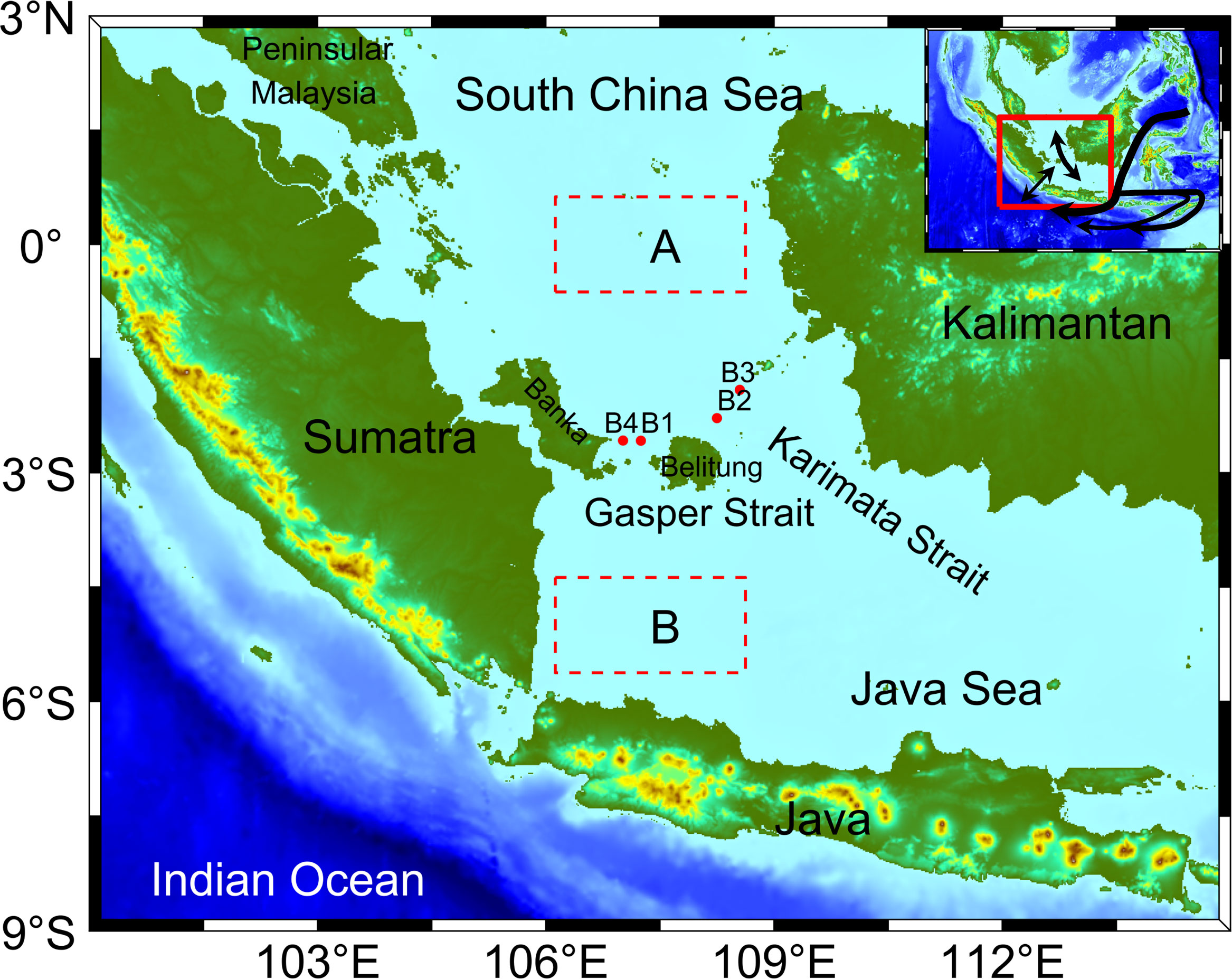
Figure 1 Study region and the observation sites in the KS. (A, B) are the areas selected to calculate the sea surface height gradient.

Research on the KS throughflow (KSTF) can be traced back to Wyrtki (1961). Using ship observational data, he found that the surface current in the KS has a seasonal reversal; it flows southward from the SCS to the JS in winter with a volume transport of -4.5 Sv (1 Sv = 10⁶ m³s^-1, positive northward), and flows northward from the JS to the SCS in summer with a volume transport of 3.0 Sv. According to model simulations, scientists determined that the KS is not only a direct connection between the SCS and Indonesian Seas (Fang et al., 2002), but also an important part of the SCS branch of the Pacific-to-Indian-Ocean throughflow (Fang et al., 2005; Qu et al., 2005; Wang et al., 2006; Yaremchuk et al., 2009; Susanto et al., 2010). The KSTF contributes to the ITF volume transport (Fang et al., 2005), accounting for 13% of the ITF annual transport (He et al., 2015). The interaction between the KSTF and ITF has also been studied using a HYCOM/FVCOM model simulation. It is found that in winter, the low-salinity water from the SCS is transported to Makassar Strait through the KSTF to block the southward ITF, whereas in summer part of the ITF is advected into the SCS through the KS with advection onto the Peninsular Malaysia’s east coast (Gordon et al., 2012; Xu and Malanotte-Rizzoli, 2013; Kok et al., 2021), and part of the inflow has a contribution to the deep meridional overturning circulation in the SCS (Shu et al., 2014).

The South China Sea-Indonesian Seas Transport/Exchange and Impact on Seasonal Fish Migration (SITE) project was launched in 2006 to directly measure variations in the KSTF through observations (Susanto et al., 2010; Wei et al., 2019). Fang et al. (2010) and Susanto et al. (2013) analyzed early data from SITE and confirmed the existence of the SCS branch of Pacific-to-Indian-Ocean throughflow through the KS with a stronger southward flow in winter and weaker northward flow in summer. They also found that bottom currents flow southward all year, although the flow was close to zero in summer. Wang et al. (2019) and Xu et al. (2021) used the long-term data from SITE to discuss the seasonal and interannual variations of KSTF and proposed that the seasonal cycle is dominant forced by the local monsoon winds and sea surface height (SSH) gradient. They also found an interannual variation with a period of 2.5-4.5 years, but without a significant correlation to the Indian Ocean Dipole (IOD) or El Niño-Southern Oscillation (ENSO).

Estimates of the KSTF annual mean transport vary considerably in the early studies, ranging from -0.3 to -4.4 Sv (Table 1). In recent years, results of both in situ observation and numerical simulation tend to fall between -0.7 and -1.0 Sv. Although the annual mean transport of the KSTF is smaller than that of the ITF, the KSTF does contribute a seasonal variability of more than 5 Sv, and plays a dual role in the total ITF volume transport (Fang et al., 2010). Combining in situ observation data with remote sensing data, Xu et al. (2021) constructed a long time series (from 1993 to 2017) of water transport through the KS that shows a strong seasonal variation (blue line in Figure 2) and a relatively weak interannual variation of annual mean transport (black line in Figure 2). In addition to these variations, the seasonal variability from year-to-year (red dotted line in Figure 2) are much greater than the interannual variability of annual mean transport (black solid line in Figure 2). Therefore, it is very important to investigate the interannual modulations of seasonal variability (Hamlington et al., 2019). In this paper, we focus on the seasonal amplitude modulations of the KSTF on interannual to decadal time scales.

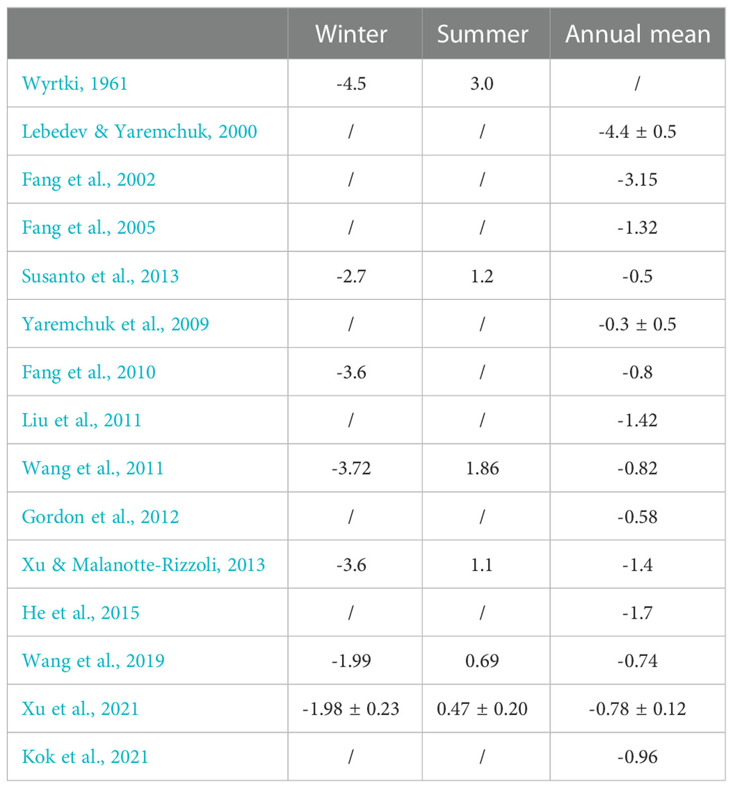
Table 1 Estimated volume transport values of KSTF (unit: Sv).

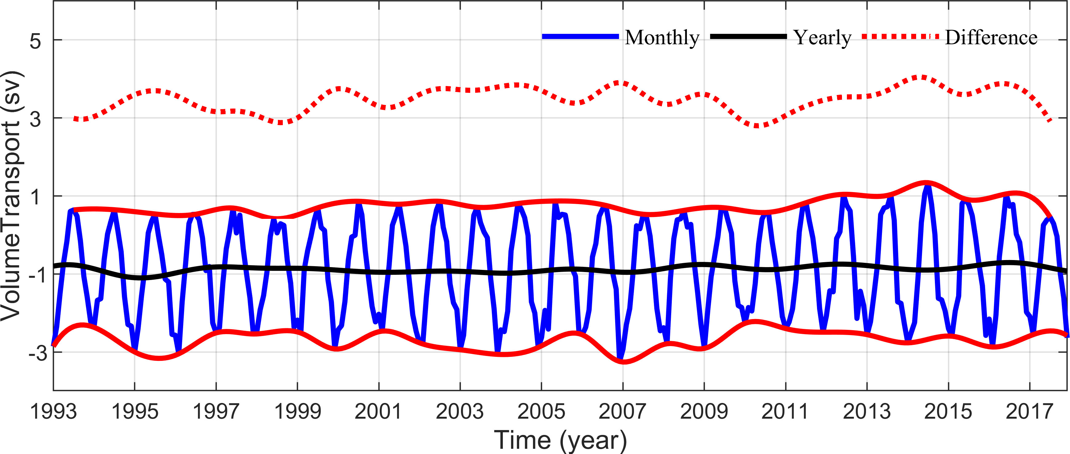
Figure 2 Time series of monthly averaged volume transport through the KS (Xu et al., 2021). Blue solid line indicates the monthly values; black solid line indicates the yearly values; red solid lines indicate the envelopes of the blue line; and red dotted line indicates the difference between red solid lines.

The rest of this article is organized as follows. Section 2 describes the satellite remote sensing and field observation data used to calculate the KS transport. Section 3 introduces the methods for multiple linear regression and calculating volume transport, heat transport, and the seasonal amplitude. In Section 4 we show the interannual to decadal modulations in seasonal amplitudes. In Section 5 we discuss the potential influencing factors for the changes in the seasonal amplitude. Summary and discussion are given in Section 6.

2 Data

2.1 Satellite remote sensing data

Even though in situ observations of the KS transport have been conducted in collaboration among scientists from Indonesia, China and USA, the observations can’t last for longtime to observe the decadal variability. Hence, the satellite remote sensing data of SST, sea surface wind (SSW), and SSH are used as proxies to study the decadal modulations in the seasonal amplitudes of the KS volume and heat transports. The SST data are NOAA 1/4° Daily Optimum Interpolation of SST (OISST) using Advanced Very High-Resolution Radiometer (AVHRR) data (Reynolds et al., 2007; Huang et al., 2021) with temporal coverage from 1981 to the present. The SSW data are derived from version 2.0 and 2.1 NRT of Cross Calibrated Multi-Plantform (CCMP) with a time resolution of 6 h and spatial resolution of 0.25° × 0.25°. The temporal coverage spans from 1987 to 2019 for version 2.0 and from 2015 to present for version 2.1 NRT (Atlas et al., 2011; Wentz et al., 2015). The SSH data are the daily gridded product processed by the DUACS multi-mission altimeter data processing system, with metadata provided by the Copernicus-Marine Environment Monitoring Service (CMEMS). The SSH data cover from 1993 to present with a spatial resolution of 0.25° × 0.25°. The monthly averages of these data from 1993 to 2021 are calculated for use in this study.

2.2 Field observation data

A series of direct current and thermohaline observations in the KS from 2007 through 2016 were supported by SITE (Wei et al., 2019). Four trawl-resistant bottom mounts (TRBMs) were deployed in the south section of the KS from November 2008 to May 2016. The locations of the four stations were: B1 (2°34.625′S, 107°15.033′E), B2 (2°16.689′S, 108°14.816′E), B3 (1°54.618′S, 108°32.703′E), and B4 (2°34.623′S, 107°0.899′E) (Figure 1). Each TRBM carried one upward-looking acoustic Doppler current profiler (ADCP) for velocity profile observations, and one conductivity-temperature-depth (CTD) recorder or tide gauge (TG) recorder to measure the temperature and pressure on the bottom. In some of these cruises, the CTD or TG was not equipped in the TRBMs; Therefore, some of the time, the bottom temperature and pressure observations were missing.

Using in situ observation current data, the velocity time series at four stations in the KS and GS are daily averaged to remove the tidal signals, and projected to the normal directions of the sections. The normal directions of the KS (B2 and B3) and the GS (B1 and B4) sections are 309° and 0° (compared to true north), respectively. Finally, the time series of the along-strait velocity (ASV) at different depth layers are obtained (Xu et al., 2021).

3 Methods

3.1 Multiple linear regression

To cope with the gaps in the field observations data, we use remote sensing data to fill the gaps and extend the time series in order to investigate interannual to decadal modulations. The KSTF is forced by local winds and along-channel sea surface slope (Fang et al., 2010; Wang et al., 2019). Therefore, we can use remote sensing data to reconstruct the KSTF with a multiple linear regression model (Formula 1). The continuous and long-term ASV time series at each station can then be obtained based on the calculated regression coefficients of all depth layers (Supplementary Table 1). This method was used to study seasonal and interannual variations in the KSTF by Fang et al. (2010), Wang et al. (2019) and Xu et al. (2021). In this study we use this method to reconstruct a long-term time series of the KSTF to investigate modulations in the KSTF seasonal amplitudes. The details are shown in Wang et al. (2019) and Xu et al. (2021). The ASV is calculated from

Where Uwnd and Vwnd represent the zonal and meridional components of the local SSW, u₀ is the magnitude of the basic current, ϵ represents the residual, and ΔADT is the difference of the regional mean SSH between the north (0.625°S - 0.625°N, 106.125°E - 108.625°E) and the south (4.375°S - 5.625°S, 106.125°E - 108.625°E) (Figure 1) parts of the KS, which were selected based on the correlation coefficients with the velocity of the KSTF (Wang et al., 2019; Xu et al., 2021). a₁ , a₂ , and a₃ are the linear regression coefficients.

3.2 Volume and heat transports

The volume transport is calculated using the following formula (Fang et al., 2010; Wang et al., 2019):

where i and k represent the row and column number of each grid in the section, respectively, Δz_k is the height of grid, Δl_i the width of grid, and v_i,k is the average normal velocity of each grid.

The heat transport is calculated as follows:

where, T_i,k and ρ_i,k represent the average temperature and density of each grid respectively. T₀ is the reference temperature, which is set to 3.72 °C (Fang et al., 2010; Kok et al., 2021), and specific heat capacity C_p is 3.89 × 10³ J kg⁻¹°C⁻¹. To accurately calculate the heat transport through the KS, the temperature profile at each station is calculated based on the bottom temperature observed from the TRBMs and the SST remote sensing data. The specific process is shown in Xu et al. (2021).

3.3 The seasonal amplitude

Seasonal amplitude is an important factor for evaluating interannual differences in seasonal cycle or seasonal variability. In this paper, we employ two methods to estimate the seasonal amplitude of the KSTF.

a) Method 1: winter and summer difference algorithm

Since the seasonal cycle is mainly shown in the difference between the winter and the summer, we can use the difference to represent the intensity of this seasonal change. Half of the absolute value of this difference is used as the seasonal amplitude value, and the difference is defined as the monthly mean minimum occurring in winter minus the average of monthly mean maximums occurring in the preceding and following summers:

where A_i+1 is the seasonal amplitude value in the i+1th year,  Min_i represents the monthly mean minimum value of a time series in winter of the ith to the i+1th year, Max_i represents the monthly mean maximum of a time series in summer of the ith year, and Max_i+1 represents the monthly mean maximum in summer of the i+1th year. These two summer averages are located on both sides of this winter. The time interval of seasonal amplitude time series calculated by this method is one year. While extracting the seasonal amplitude of SST, Max_i and Max_i+1 represent the monthly mean maximums of the ith year and the i+1th year, respectively.

b) Method 2: harmonic algorithm

The annual cycle is predominantly characterized by harmonic oscillations. Therefore, the harmonic parameters of the annual cycle can be estimated to study modulations in seasonal variability on interannual to decadal scales. Reconstructed KSTF is harmonically analyzed in 2-year windows at monthly time steps (Formula 5). The 2-year window is selected because it can maintain a better continuity of results and show subtle changes in the annual cycle, while minimizing the interference of high-frequency changes (Hamlington et al., 2019). The fitting step involves solving the least squares function to obtain the optimal linear trend and annual harmonics (Chandanpurkar et al., 2021). The value obtained from each fitting is assigned to the intermediate time.

where t, a and b are time, intercept, and linear slope respectively, c and d represent the amplitude of annual harmonic cosine and sine component respectively, and ω represents frequency of annual period. The seasonal amplitude A can be obtained by the formula below. The time interval of seasonal amplitude time series by this method is one month. The seasonal amplitude is defined as half of the difference between peak and trough, which is half of that from Chandanpurkar et al. (2021).

Both methods show the intensity of seasonal variability, however, Method 1 mainly shows the difference between winter and summer and Method 2 shows the whole annual cycle. Therefore, the seasonal amplitudes obtained using Method 1 are slightly larger than those obtained using Method 2. In addition, the time resolution for the results of Method 1 is one year, and it is one month for Method 2. Method 1 accurately describes the interannual variation of seasonal amplitude time series, while Method 2 has a potential role of smoothing the seasonal amplitude time series.

4 Interannual to decadal modulations in seasonal amplitude

4.1 The seasonal amplitudes of currents and SST

Using the multiple linear regression model described in the Section 3.1, the 29-year ASV time series of each layer at four stations in the KS are obtained from satellite remote sensing and field observation data. The vertically-averaged ASV time series at four stations in the KS show a dominant seasonal variation (Figure 3A). However, there are also significant interannual modulations in the seasonal amplitudes. Figures 3B and 3C show the seasonal amplitudes of vertically-averaged ASV time series at four stations derived by the two methods given in the Section 3.3. The results of winter and summer difference algorithm (Method 1) are shown in Figure 3B. Meanwhile, Figure 3C shows the seasonal amplitudes calculated by the harmonic algorithm (Method 2). It can be seen that the fluctuations in the seasonal amplitudes of the vertically-averaged ASVs at four stations are synchronized, with the highly consistent modulation ranges. The trends in the seasonal amplitudes of the velocities at different stations in the KS are consistent. All of them reach their minimum during the periods of 1997-1999, 2010-2011, and 2017-2018, and reach their maximum during 1995-1996, 2002-2004, and 2014-2016. Compared with the results obtained by Method 1, the seasonal amplitude time series from Method 2 are smoother and have a higher time resolution, clearly showing the interannual to decadal modulations.

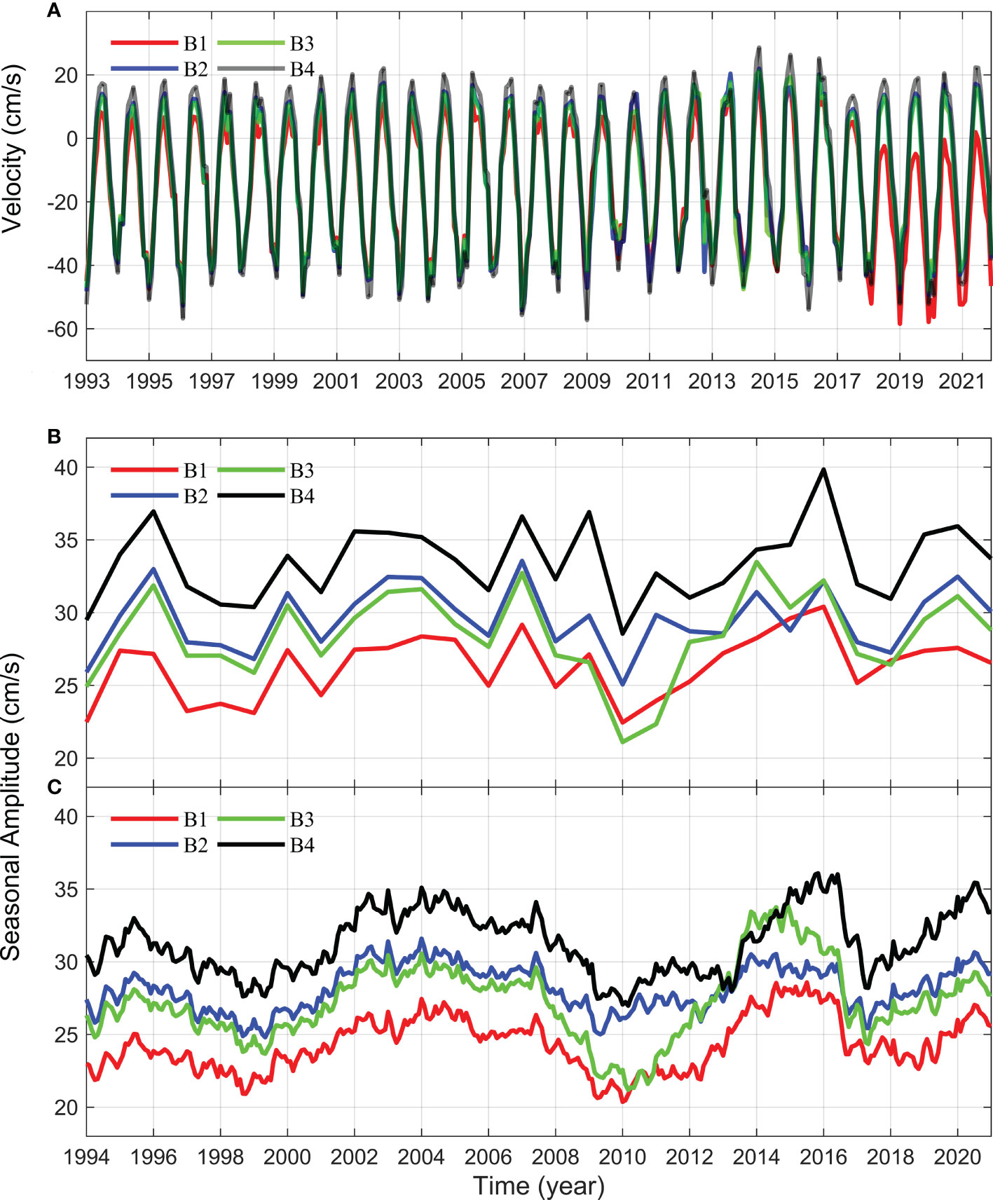
Figure 3 (A) Time series of vertically-averaged ASVs at four stations. (B) The seasonal amplitudes of vertical average ASVs obtained by the winter-summer difference algorithm (Method 1), (C) same as (B) but by the harmonic algorithm (Method 2).

By comparing the seasonal amplitudes calculated by the two methods (Figure 3 and Table 2), we note that the results obtained by different methods at same station are basically consistent in the means, ranges, and trends. This confirms the validity of the two methods to calculate the seasonal amplitude. The seasonal amplitude of the vertically-averaged ASV at B4 is always the largest, followed by B2 and B3. The amplitude at B1 is smallest, which is related to the stronger flow in the western strait. When the western boundary current of the SCS flows southward into the KS near the equator, it retains its characteristics of westward strengthening. This may be caused by the inertance of flow, as the westward intensification effect near the equator is always ignored (Fang et al., 2005). In general, the seasonal amplitude based on Method 1 are higher than that from Method 2, with an average value of 1.70 ± 0.45 cm s^-1 higher for each of the four stations. Whereas the ranges are basically the same, with a difference of less than 0.80 cm s^-1.

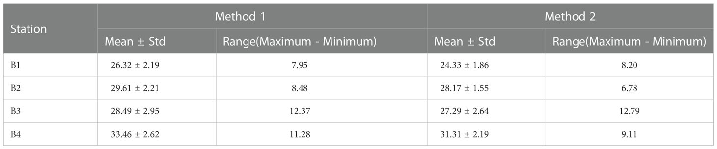
Table 2 The mean and range of seasonal amplitude of velocity (unit: cm s^-1).

Given that the KSTF plays an important role in the heat budget of the SCS and ITF heat transport (Qu et al., 2005; Tozuka et al., 2007; Tozuka et al., 2009; Zeng and Wang, 2009; Fang et al., 2010; Gordon et al., 2012), it is important to investigate SST variation in the KS except for the current velocity. The monthly SST time series in the KS (Figure 4A) is obtained by averaging the SST data at the four stations. In contrast to the time series for current, the SST time series have not only annual cycle, but also semi-annual cycle. However, we are still able to use Method 1 and Method 2 to calculate the seasonal amplitude. The seasonal amplitudes of SST (Figures 4B, C) and current velocity are all not synchronized. When the seasonal amplitude of velocity is at a maximum or minimum, there is no corresponding change in SST. The seasonal amplitude of SST has a more significant interannual signal than that of current. There are decreasing trends of -0.08 ± 0.13 and -0.10 ± 0.02 °C decadal^-1 in the seasonal amplitudes obtained using Method 1 and Method 2.

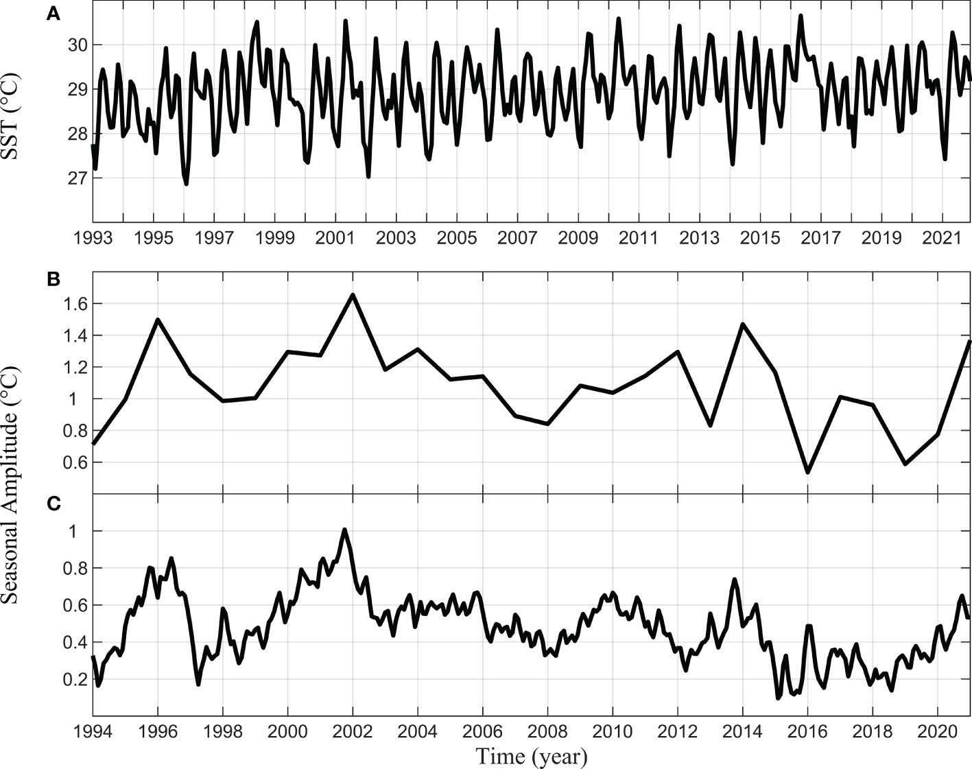
Figure 4 (A) Time series of monthly average SST data. (B) The seasonal amplitude of SST obtained by the winter-summer difference algorithm (Method 1), (C) same as (B) but by the harmonic algorithm (Method 2).

4.2 The seasonal amplitudes of volume and heat transports

In order to quantitatively evaluate modulations in the seasonal amplitude of the KSTF, the KS volume transport is firstly calculated according to Formula 2 (Figure 5A). During 1993-2021, the annual mean volume and heat transports through the KS are -0.76 ± 0.08 Sv and -71.23 ± 7.42 TW (1 TW = 10¹² W), respectively. These values are similar to the annual average of -0.78 ± 0.12 Sv and -77.31 ± 4.99 TW from 1993 to 2017 reported by Xu et al. (2021). This confirms that the reconstructed monthly averaged time series of volume transport is reliable. The interannual variation is obtained by removing the seasonal variation from the monthly averaged time series of volume transport using a 3-year low-pass filter (Figure 5B). During 1993-2004 and 2005-2017, there are rapid changes in the volume transport, implying an enhancement and a decay in the southward total transport with linear trends of -10.10 ± 3.20 and 6.29 ± 2.18 mSv year^-1 (1 mSv = 10³ m³s^-1), respectively.

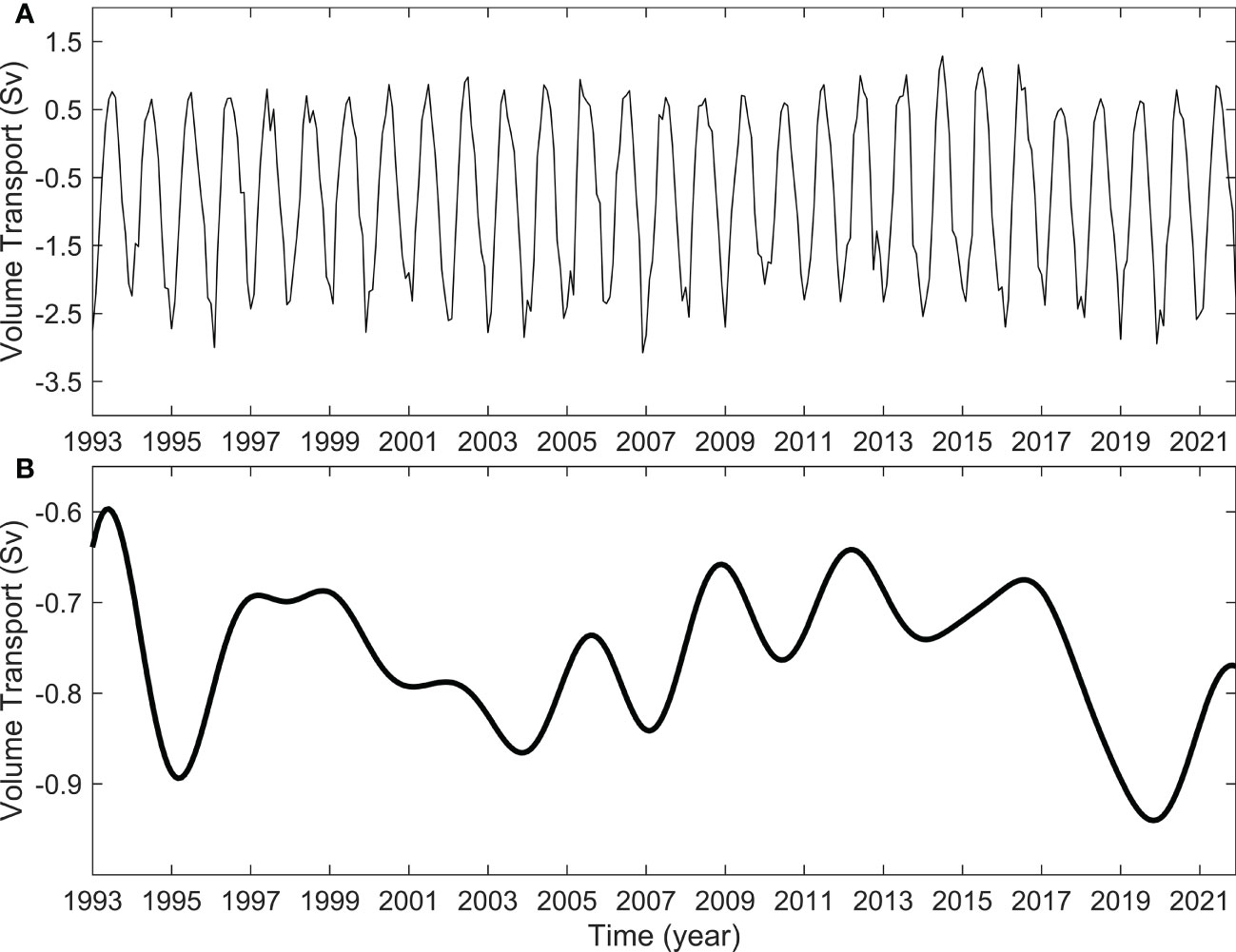
Figure 5 (A) Monthly mean volume transport through the KS sections, and (B) the interannual variation obtained using a 3-year low-pass filter.

Because the seasonal amplitude of volume transport can describe the intensity of seasonal variability in the KSTF, we can use two methods mentioned in Section 3.3 to extract seasonal amplitude from the transport time series. As shown in Figure 6, the seasonal amplitudes of the KS volume transport calculated using the two methods result in long-term and linearly increasing trends of 28.27 ± 67.10 and 37.75 ± 15.69 mSv decade^-1. This data suggests that from 1994 to 2020 the difference in transport between winter and summer is gradually increasing. The water exchange between the SCS and the JS through the KS is in an enhanced state, thus affecting the hydrological characteristics of two areas, and also have an impact on the water transport and seasonal variation of ITF (Tozuka et al., 2007; Tozuka et al., 2009; Fang et al., 2010; Gordon et al., 2012; Li et al., 2021). Moreover, it can be seen that the time series obtained by the two methods are generally consistent with each other and show similar interannual to decadal modulations that range between 1.36 and 1.92 Sv. The seasonal amplitudes obtained using the two methods both reach the maximum during 1995-1996, 2003-2004, 2014-2015, and minimum during 1998-1999, 2009-2010, 2016-2017. Due to the low time resolution of Method 1 and the smoothing effect of Method 2, there are some other extreme points ignored in Figure 6A. The average seasonal amplitudes obtained using the two methods separately are 1.69 ± 0.14 and 1.60 ± 0.12 Sv, which are much larger than the annual mean value of water transport through KS, -0.76 ± 0.08 Sv. This indicates that seasonal variability and its amplitude modulations play important roles in KSTF transport, and it can reverse the KSTF in different season.

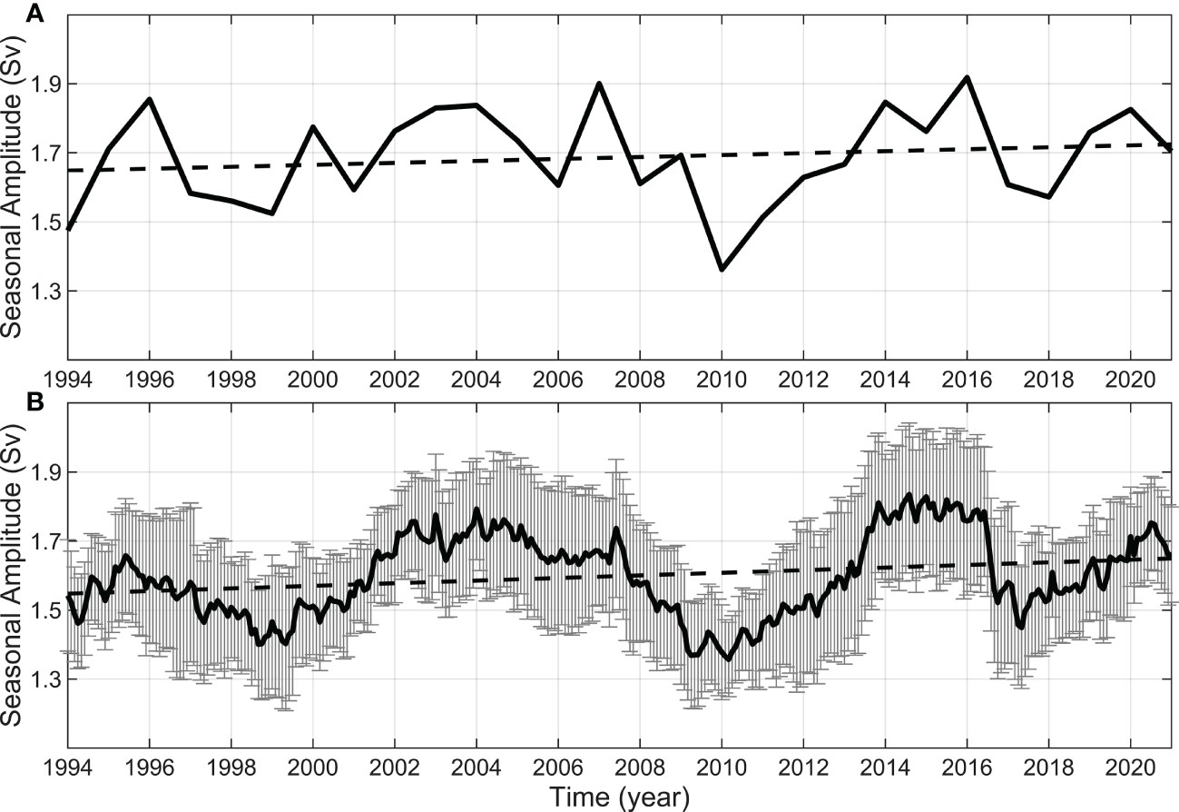
Figure 6 The seasonal amplitude of the KS volume transport obtained (A) by the winter-summer difference algorithm (Method 1), (B) by the harmonic algorithm (Method 2). Black solid line indicates the seasonal amplitude values, and black dotted line indicates the linear fitting values.

The time series of heat transport through the KS is calculated using Formula 3. Next the time series of seasonal amplitude (Figure 7) is extracted using Formula 5 (Method 2). It can be seen that the trend in the seasonal amplitude of heat transport is almost consistent with that of volume transport. This implies that the current variation plays a more important role than the temperature variation. The seasonal amplitude of heat transport ranges between 126.41 and 173.36 TW, with an average value of 148.89 ± 11.47 TW. Similar to the volume transport, the seasonal amplitude of heat transport shows similar periodic changes. The linear fitting results in a gradually increasing trend with rising variability of 4.78 ± 1.52 TW decade^-1. This increasing trend in seasonal amplitude of heat transport represent an enhancement in the heat exchange between the SCS and the JS, which influences not only the heat content of the two seas, but also the ITF heat transport.

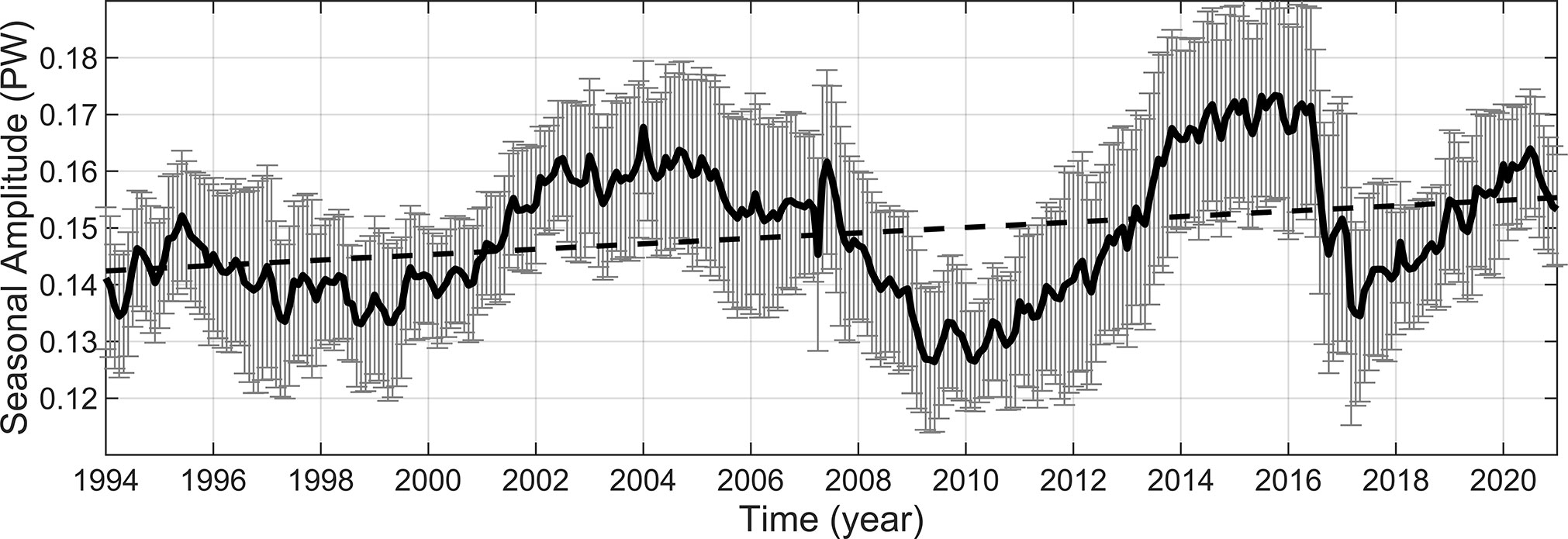
Figure 7 The seasonal amplitude of the KS heat transport obtained by the harmonic algorithm (Method 2). Black solid line indicates the seasonal amplitude values, and black dotted line indicates the linear fitting values.

In addition to linear trends, the seasonal amplitude time series of volume and heat transports also show periodic fluctuations (Figures 6, 7). The results by power spectrum analysis are shown in Figure 8. It can be seen that there are prominent interannual to decadal signals with the typical periods of ~9 and ~13.5 years for the seasonal amplitude time series of heat transport, and ~9 years for the volume transport. which are all above the 95% confidence level. According to the results obtained using the Method 2, the correlation coefficient between the two transports seasonal amplitude time series is up to 0.98 (above the 95% confidence level).

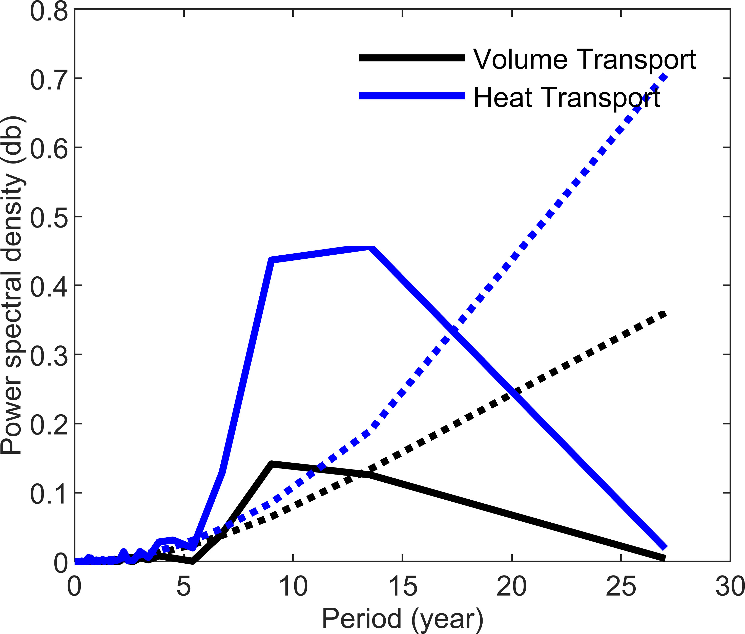
Figure 8 Power spectrum of the seasonal amplitude time series of volume and heat transports. The black solid line represents the result of volume transport, and the black dotted line represents its 95% confidence level; the blue solid line represents the result of heat transport, and the blue dotted line represents its 95% confidence level.

4.3 Contributions to the seasonal amplitude of heat transport

The velocity and temperature of the KS sections can be decomposed into seasonal cycles and anomalies ( $V=\overline{V}+V^{\prime }$, $T=\overline{T}+T^{\prime }$). Therefore, the formula for heat transport can be written as Formula 7 (Xu et al., 2021). The first three items on the right of the formula represent the contributions of climatologic state, velocity change, and temperature change, while the fourth term is a high-order term. For convenience, the water density is set as 1024 kg m^-3. Figure 9 shows the seasonal amplitude time series of the four terms, where velocity and temperature anomalies both contribute to the interannual to decadal modulations in the seasonal amplitude of heat transport, accounting for 6.25 and 0.88 TW, respectively. The primary contribution to the amplitude modulations in seasonal heat transport is the velocity anomaly, followed by temperature anomaly. The velocity anomalies trigger an increasing trend of 2.11 ± 0.84 TW decade^-1 of the seasonal amplitude of heat transport from 1994 to 2020, and the temperature anomalies induce a decreasing trend of -0.26 ± 0.12 TW decade^-1 in the seasonal amplitude of heat transport.

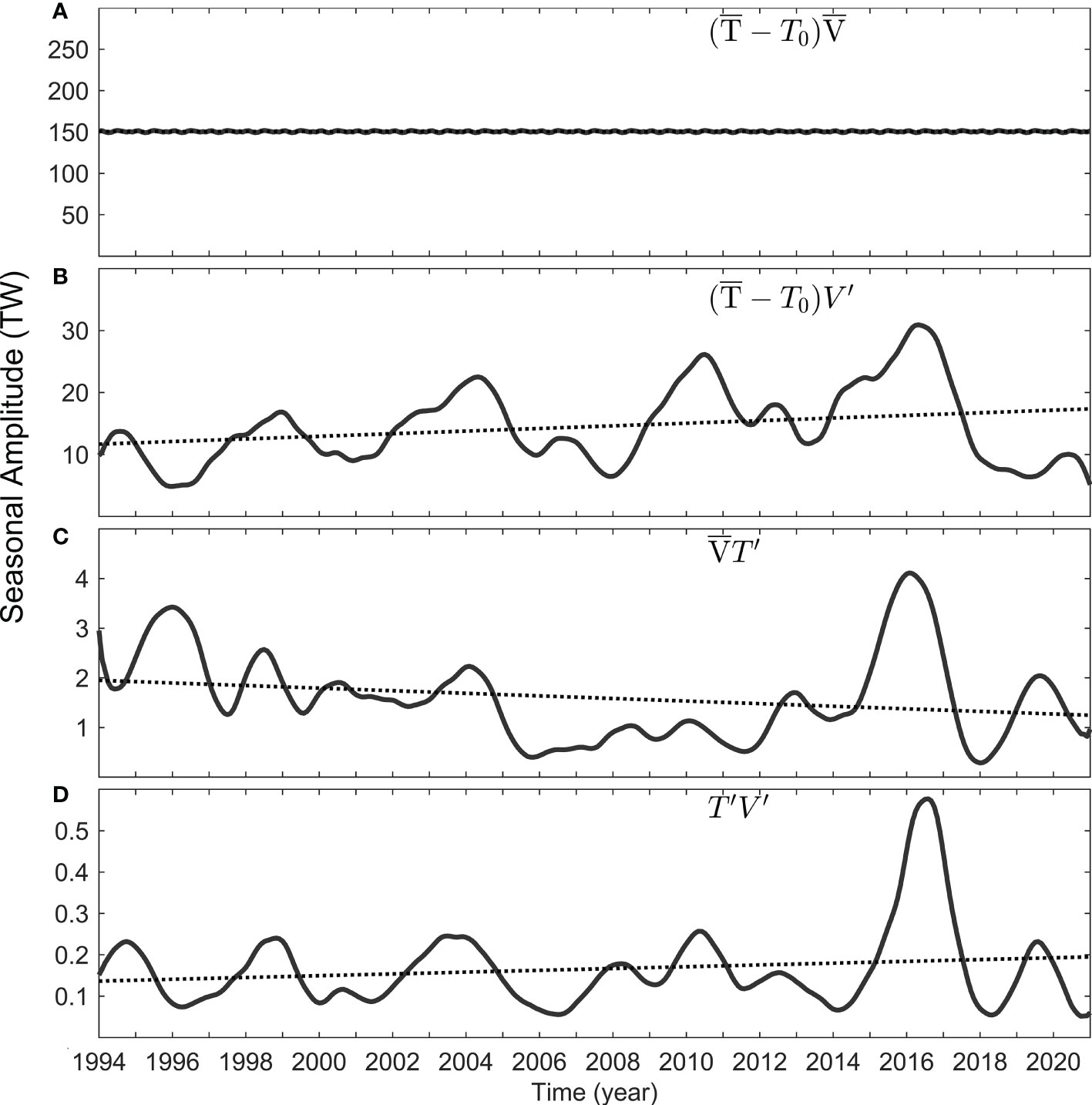
Figure 9 The Seasonal amplitude time series of (A) climatologic state, (B) velocity anomaly, (C) temperature anomaly, and (D) higher-order terms in the formula of heat transport. These seasonal amplitudes are extracted using the harmonic algorithm (Method 2). The time series in (B), (C), and (D) are smoothed by 13-month moving average before plotting.

5 Potential influencing factors on changes in the seasonal amplitude

5.1 Relationships with SSH and SSW

The KSTF is mainly forced by the local SSW field and along-channel SSH gradient in the KS (Wang et al., 2019; Xu et al., 2021), therefore, we can calculate the seasonal amplitudes of SSW and SSH and analyze the relationship between them (Figure 10). The results show that the fluctuations in the interannual modulations of the SSH gradient, local meridional SSW, and volume transport are highly consistent. Meanwhile the modulations in local zonal wind are relatively independent. The average seasonal amplitudes of SSH gradient, local meridional wind, and local zonal wind are 0.17 ± 0.01 m, 3.93 ± 0.45 m s^-1, and 4.16 ± 0.40 m s^-1, respectively. The partial correlation coefficients of the SSH gradient, local meridional and zonal winds with the volume transport seasonal amplitude are 0.72, 0.65 and 0.02, respectively. The first two correlations are significant at the 95% confidence level, but the local zonal wind is not. This indicates that interannual to decadal signals of seasonal amplitude also exist in the SSH gradient and local SSW field, and the SSH gradient and meridional component of local SSW fields are the main contributors to the volume transport seasonal amplitude. In addition, during 1994-2020 there is a upward trend of 0.25 ± 0.06 m s^-1decade^-1 in seasonal amplitude of local meridional wind, which is above the 95% confidence level. The trends in seasonal amplitudes of the SSH gradient and local zonal wind are -0.19 ± 0.17 cm decade^-1 and 0.06 ± 0.05 m s^-1decade^-1 respectively, which are not significant.

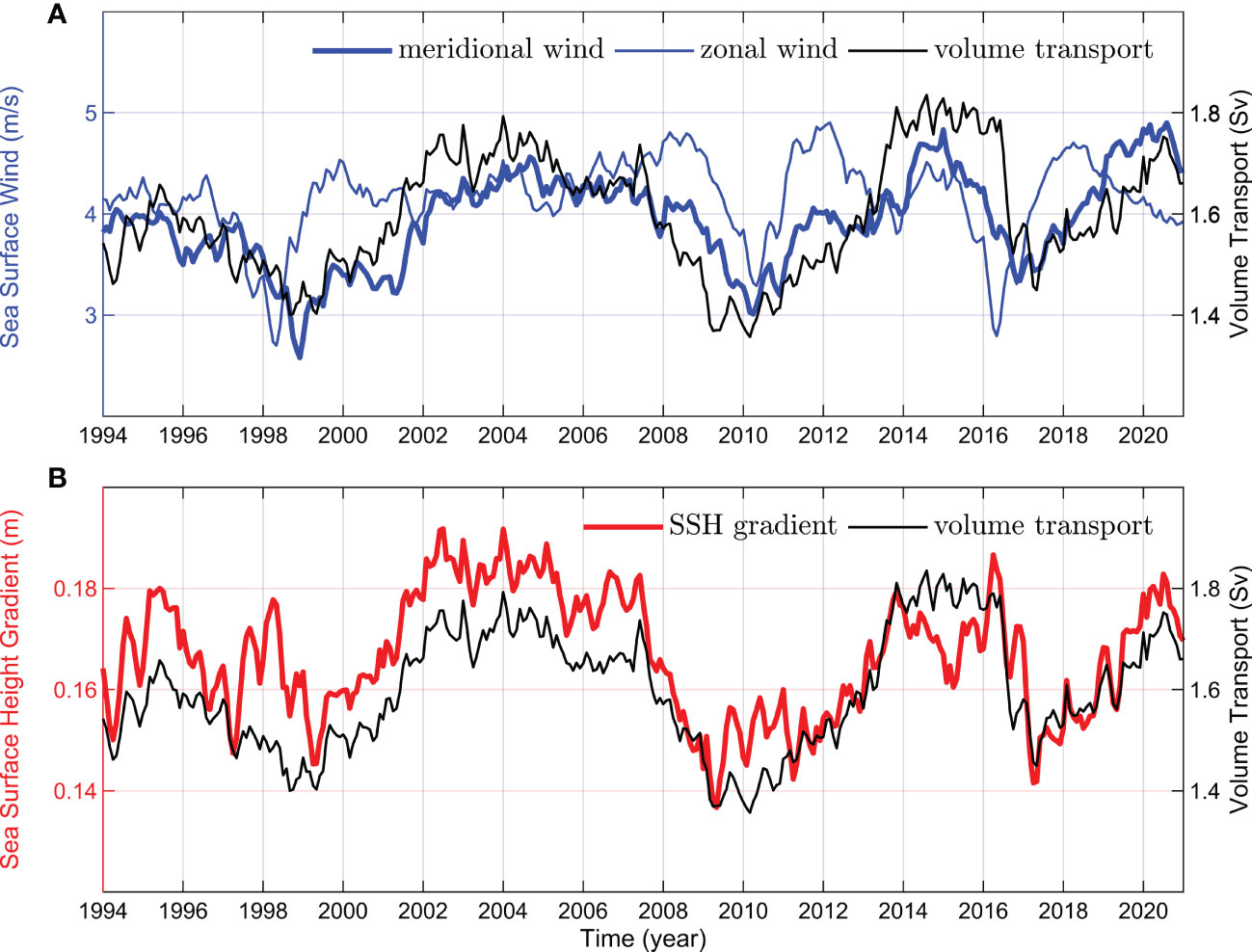
Figure 10 (A) Seasonal amplitudes of local meridional (blue thick line) wind field, zonal (blue thin line) wind field and volume transport (black solid line) obtained by harmonic algorithm (Method 2). (B) Seasonal amplitudes of SSH gradient (red solid line) and volume transport (black solid line) obtained using the harmonic algorithm (Method 2).

5.2 Relationships with ENSO, IOD, and the Pacific decadal oscillation

In previous studies on the annual mean variation of the KS, Gordon et al. (2012) and Xu et al. (2021) pointed out that the interannual variability of KSTF had an insignificant correlation with ENSO and IOD. Other studies have suggested that the interannual variability of the KSTF was modulated by ENSO and IOD (Du and Qu, 2010; He et al., 2015). In this study, we explain the interannual to decadal modulations in the KS from the perspective of seasonal amplitude and analyze correlations between the KSTF and the ENSO, IOD, and Pacific Decadal Oscillation (PDO). The Niño3.4 index, used to characterize the intensity of the ENSO is downloaded from https://psl.noaa.gov/data/timeseries/monthly/NINO34/. The strength of the IOD measured using the Dipole Mode Index (DMI) defined by Saji and Yamagata, 2003, is downloaded from https://psl.noaa.gov/gcos_wgsp/Timeseries/DMI/. The PDO index, defined by Deser et al. (2016), is obtained from https://www.ncei.noaa.gov/access/monitoring/pdo/. Figure 11 shows the seasonal amplitude time series of volume transport and these climate indices. Since Method 2 (harmonic algorithm) has the function of moving average while extracting the seasonal amplitude, these indices are processed with 24-month running mean.

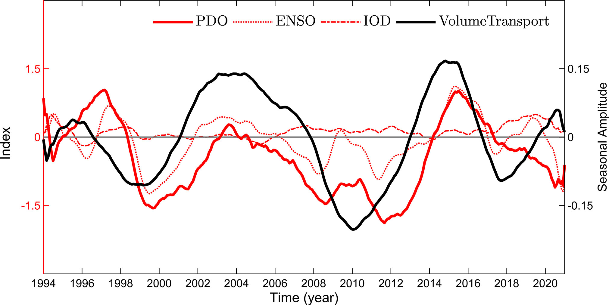
Figure 11 Relationships between the seasonal amplitude of volume transport and the ENSO, IOD, and PDO, where these indices have passed a 24-month running mean. The seasonal amplitude of volume transport obtained by the harmonic algorithm (Method 2) is the black solid line which is detrended; PDO index is the red solid line; Niño3.4 index is the red dashed line; DMI index is the red dot-dashed line.

From the Figure 11, it can be seen that the seasonal amplitude of volume transport is consistent with the low-frequency variation of the ENSO and the PDO, but different from the IOD. The cross-correlations between the seasonal amplitude of volume transport and climate indices are carried out to understand the lead and lag time of the climate events. When the PDO, ENSO, and IOD events lag behind the seasonal amplitude by 12, 10, and 3 months, the correlation coefficients reach maximum values of 0.69, 0.58, and -0.38 (above the 95% confidence level), respectively. Qin et al. (2016) noted that the pressure difference between the West Pacific and East Indian Ocean is closely correlated to the KS transport on the decadal scale. The variability of the pressure difference is primarily controlled by the variability of SSH in the East Indian Ocean, which appears to be modulated by PDO.

5.3 Composite analysis results

Since the seasonal amplitudes of water transport has a good correlation with the PDO, we use composite analysis to investigate the differences in SSH and SSW of the adjacent seas during different phases of the PDO. The warm PDO phases are identified as 1996, 1997, 2003, 2004, 2014, and 2015, and the cold PDO phases are identified as 1998, 1999, 2010, and 2011 (Figure 11). Figures 12A–C show the composite analysis results of SSH and SSW field in winter, in summer and their difference in warm PDO phases. Figures 12D–F show the same information for cold PDO phases. The local meridional wind and the difference in regional mean SSH between the north and south areas of the KS (see Section 3.1) are calculated during these two phases.

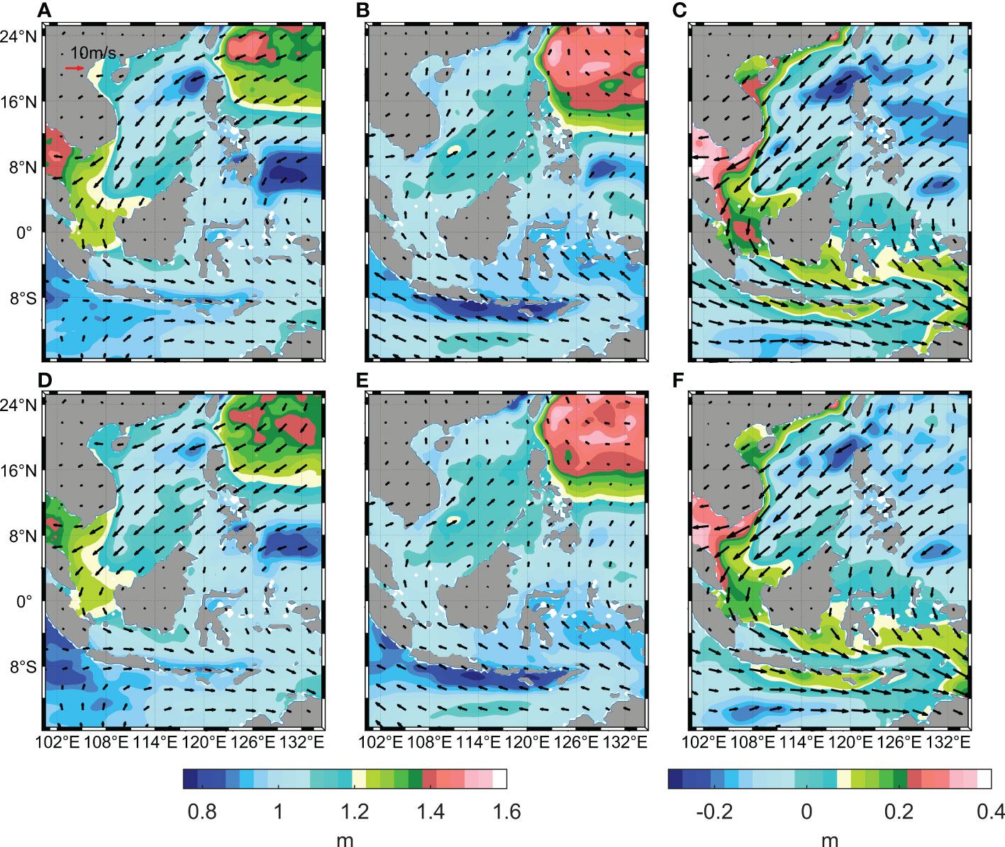
Figure 12 Composite analysis results of SSH and SSW field in winter (A) and summer (B) and the seasonal amplitude (C) in warm PDO phases. Composite analysis results of SSH and SSW field in winter (D) and summer (E) and the seasonal amplitude (F) in cold PDO phases.

During winter of warm PDO phases (Figure 12A), the northerly wind from the SCS reaches the KS with strong wind speed. The meridional component of the wind reaches up to -4.41 m s^-1 while the along-channel SSH slope is about -27.89 cm. However, the SSW over the SCS in winter of the cold PDO phases is more easterly compared to that of the warm PDO phases (Figure 12D). This easterly SSW induces a substantial decrease to -2.92 m s^-1 in the meridional wind over the KS, accompanying a decrease to -24.74 cm in the along-channel SSH slope. In summer during warm and cold PDO phases (Figures 12B, E), the southeast monsoon from the Indian Ocean covers the KS after crossing the JS. However, the differences in local meridional wind and SSH slope between that of two phases are only 0.04 m s^-1 and 0.79 cm, respectively. Therefore, there are significant differences of the local SSW and SSH slope between warm and cold PDO phases in winter, but not in summer. Figures 12C, F show the winter-summer differences of the SSW and SSH in warm and cold PDO phases, respectively. The results indicate that the seasonal amplitudes of the local SSW and SSH slope in KS are stronger in warm PDO phases than that in cold PDO phases. As the ENSO displays low-frequency variability that is similar with the PDO (Newman et al., 2003; McGregor et al., 2010), the composite analysis results are consistent during the ENSO and PDO phases.

6 Summary and discussion

The variability in the seasonal Karimata Strait (KS) transport is often assumed to be time-invariant, however, it changes from one year to the next and needs a modified characterization to account for its variations. Therefore, it is necessary to investigate the amplitude modulations in seasonal KS throughflow (KSTF).

In this study, we use two methods (the winter-summer difference algorithm and harmonic algorithm) to calculate the seasonal amplitude of the KSTF based on the reconstructed time series of transports from 1993 to 2021. The results calculated by these two methods show the same significant interannual to decadal modulations in the seasonal amplitude of the KSTF. In general, the modulations in the seasonal amplitude of volume transport obtained by these two methods are consistent, both ranging between 1.36 and 1.92 Sv. The average seasonal amplitudes of the volume transport calculated using the two methods are 1.69 ± 0.14 and 1.60 ± 0.12 Sv, respectively, which are double the size of the annual mean volume transport. Meanwhile, there are increasing trends in them with rates of 28.27 ± 67.10 and 37.75 ± 15.69 mSv decade^-1, respectively. If the linear trend is still increasing in future, it implies that the KSTF would be significantly strengthened in winter or summer. The average seasonal amplitude of heat transport calculated by harmonic algorithm is 148.89 ± 11.47 TW, with an increasing trend of 4.78 ± 1.52 TW decade^-1. The seasonal amplitude of heat transport also exhibits significant modulations, ranging between 126.41 and 173.36 TW. The seasonal amplitudes of volume and heat transports both show a quasi-period of ~9 years, and the heat transport also has a significant quasi-period of ~13.5 years. The quasi-decadal signals are similar to a global mode with 10-12 years periodicities (Feliks et al., 2021). The overall increasing trends in the seasonal amplitudes of volume and heat transports indicate that the water exchange between the SCS and the JS is gradually strengthening, which directly affects the variation range of the heat/salt content in the two seas as well as the transports and seasonal variation of the ITF. The KSTF seasonally influences the surface Makassar ITF (Wei et al., 2016; Jiang et al., 2019), therefore, the interannual to decadal modulations in the seasonal amplitude of the KSTF would result in the corresponding variations in the seasonality of the surface ITF. In winter, the KSTF not only contributes directly to the heat and freshwater transports of the ITF, but also blocks the southward Makassar ITF through the “freshwater plug” effect (Gordon et al., 2012; Xu et al., 2021). In summer, the water from the JS flows into the southern SCS through the KS. Therefore, when the KSTF transport is enhanced in winter, the seasonal variability of ITF is uncertain by dual effect. When the KS transport increases in summer, this may be accompanied by a strengthened southward surface flow in the Makassar Strait, which enhances the seasonal ITF.

The partial correlation coefficients of the SSH gradient, local meridional and zonal winds with the seasonal amplitude of the volume transport are 0.72, 0.65 and 0.02, respectively. SSH gradient and local meridional wind are significant above 95% confidence level. This indicates that interannual to decadal signals in the seasonal amplitude of the volume transport has a high correlation with that of the SSH gradient and local meridional wind, but is independent on the local zonal wind. The SSH gradient and meridional component of local SSW field are the main contributors to the seasonal amplitude of the volume transport. In addition, we note a significant increasing trend of 0.25 ± 0.06 m s^-1decade^-1 in seasonal amplitude of local meridional wind during 1994-2020, but the linear trends in the SSH gradient and local zonal wind are not significant. Therefore, the local meridional wind plays an important role in the strengthening of seasonal KSTF during 1994-2020.

PDO, ENSO and IOD lag behind the seasonal amplitude of volume transport by 12, 10 and 3 months with the correlation coefficients up to the maximum values of 0.69, 0.58 and -0.38. The KS transport is highly positively correlated with the ENSO and PDO as they have the same quasi-decadal modulations. However, there is no interannual signals of 2-5 years in the seasonal amplitude like the ENSO. According to the results of the composite analysis, in winter of the warm PDO phases, the stronger monsoon wind from the SCS reaches the KS, resulting in a large along-channel SSH slope, and intensifying the southward KSTF. In summer of the warm PDO phases, the southeast trade wind comes from the southeast Indian Ocean and the larger SSH slope induces a stronger northward KSTF. The situations are opposite during the cold PDO phases. Furthermore, the seasonality of the KS transport is significantly modulated by the quasi-decadal variations of SSH and SSW, especially in winter. Meanwhile, this quasi-decadal modulation would influence the ITF transport through the dual effect.

Data availability statement

The satellite SST data is available at https://www.psl.noaa.gov/data/gridded/data.noaa.oisst.v2.highres.html. The SSH data is available at https://marine.copernicus.eu/. CCMP Version-2.0 and Version-2.1 vector wind analyses are produced by Remote Sensing Systems, and data are available at www.remss.com. The bathymetry ETOPO1 data are available at http://www.ngdc.noaa.gov/mgg/global. The SITE data are available online https://github.com/xutengfei0207/SITE/blob/main/SITEDATA.Zip.

Author contributions

SL convinced the work, and YN performed the data analysis and wrote the original manuscript. SL and YN improved the manuscript. All authors discussed and contributed to the writing. All authors contributed to the article and approved the submitted version.

Funding

This study is jointly supported by Laoshan Laboratory (No. LSKJ202202700 and LSKJ202201904), China-Indonesia Maritime Cooperation Fund for ICCOC Development, MNR Program on Global Change and Air-Sea interactions (Contact No. GASI-04-WLHY-03), the National Natural Science Foundation of China (Grant Nos. 41876027, 41876029 and 42076023), and the Global Change and Air-Sea Interaction II (Contact No. GASI-01-ATP-STwin). RS was supported by the US National Science Foundation grant# OCE-07-25935 and the Office of Naval Research Grant # N00014-08-01-0618 through the Columbia University, New York.

Acknowledgments

We sincerely thank the captain and crews of Baruna Jaya IV, I and VIII for their skillful operation during the voyages, and we sincerely thank all the participants in the SITE cruises.

Conflict of interest

The authors declare that the research was conducted in the absence of any commercial or financial relationships that could be construed as a potential conflict of interest.

Publisher’s note

All claims expressed in this article are solely those of the authors and do not necessarily represent those of their affiliated organizations, or those of the publisher, the editors and the reviewers. Any product that may be evaluated in this article, or claim that may be made by its manufacturer, is not guaranteed or endorsed by the publisher.

Supplementary material

The Supplementary Material for this article can be found online at: https://www.frontiersin.org/articles/10.3389/fmars.2023.1085032/full#supplementary-material

References

Atlas R., Hoffman R. N., Ardizzone J., Leidner S. M., Jusem J. C., Smith D. K., et al. (2011). A cross-calibrated, multiplatform ocean surface wind velocity product for meteorological and oceanographic applications. Bull. Am. Meteorol. Soc. 92 (2), 157–174. doi: 10.1175/2010bams2946.1
Chandanpurkar H. A., Reager J. T., Famiglietti J. S., Nerem R. S., Chambers D. P., Lo M. H., et al. (2021). The seasonality of global land and ocean mass and the changing water cycle. Geophys. Res. Lett. 48 (7), e2020GL091248. doi: 10.1029/2020gl091248
Deser C., Trenberth K., Staff, N. C. F. A. R (2016). The climate data guide: Pacific decadal Oscillation(PDO): Definition and indices. NC f. a. research. doi: 10.4135/9781446247501.n2786
Du Y., Qu T. (2010). Three inflow pathways of the Indonesian throughflow as seen from the simple ocean data assimilation. Dyn. Atmosph. Oceans 50 (2), 233–256. doi: 10.1016/j.dynatmoce.2010.04.001
Fang G., Susanto R. D., Soesilo I., Zheng Q. A., Qiao F., Wei Z. (2005). A note on the south China Sea shallow interocean circulation. Adv. Atmosph. Sci. 22 (6), 946–954. doi: 10.1007/BF02918693
Fang G., Susanto R. D., Wirasantosa S., Qiao F., Supangat A., Fan B., et al. (2010). Volume, heat, and freshwater transports from the south China Sea to Indonesian seas in the boreal winter of 2007–2008. J. Geophys. Res. 115, C12020. doi: 10.1029/2010JC006225
Fang G., Wei Z., Huang Q. (2002). Volume, heat and salt transports between the southern south China Sea and its adjacent waters, and their contribution to the Indonesian throughflow. Oceanol. Limnol. Sin. (in Chinese) 33 (3), 296–302.
Feliks Y., Small J., Ghil M. (2021). Global oscillatory modes in high-end climate modeling and reanalyses. Climate Dyn. 57 (11), 3385–3411. doi: 10.1007/s00382-021-05872-z
Gordon A. L., Huber B. A., Metzger E. J., Susanto R. D., Hurlburt H. E., Adi T. R. (2012). South China Sea throughflow impact on the Indonesian throughflow. Geophys. Res. Lett. 39 (11), L11602. doi: 10.1029/2012GL052021
Gordon A. L., Susanto R. D., Vranes K. (2003). Cool Indonesian throughflow as a consequence of restricted surface layer flow. Nature 4256960, 824–828. doi: 10.1038/nature02038
Hamlington B. D., Reager J. T., Chandanpurkar H., Kim K. Y. (2019). Amplitude modulation of seasonal variability in terrestrial water storage. Geophys. Res. Lett. 46 (8), 4404–4412. doi: 10.1029/2019GL082272
He Z., Feng M., Wang D., Slawinski D. (2015). Contribution of the karimata strait transport to the Indonesian throughflow as seen from a data assimilation model. Continental Shelf Res. 92, 16-22. doi: 10.1016/j.csr.2014.10.007
Huang B., Liu C., Banzon V., Freeman E., Graham G., Hankins B., et al. (2021). Improvements of the daily optimum interpolation Sea surface temperature (DOISST) version 2.1. J. Climate 34 (8), 2923–2939. doi: 10.1175/JCLI-D-20-0166.1
Jiang G., Wei J., Malanotte-Rizzoli P., Li M., Gordon A. L. (2019). Seasonal and interannual variability of the subsurface velocity profile of the Indonesian throughflow at makassar strait. J. Geophys. Res: Oceans 124, 9644–9657. doi: 10.1029/2018jc014884
Kok P. H., Wijeratne S., Akhir M. F., Pattiaratchi C., Roseli N. H., Mohamad Ali F. S. (2021). Interconnection between the southern south China Sea and the Java Sea through the karimata strait. J. Mar. Sci. Eng. 9 (10), 1040. doi: 10.3390/jmse9101040
Lebedev K. V., Yaremchuk M. I. (2000). A diagnostic study of the Indonesian throughflow. J. Geophys. Res: Oceans 105 (C5), 11243–11258. doi: 10.1029/2000JC900015
Liu Q., Feng M., Wang D. (2011). ). ENSO-induced interannual variability in the southeastern south China Sea. J. Oceanog. 67 (1), 127–133. doi: 10.1007/s10872-011-0002-y
Li S., Xu T., Sun J., Yang L., Teng F., Wang G., et al. (2021). The interaction between the karimata strait throughflow and the Indonesian throughflow. Adv. Mar. Sci. (in Chinese) 39 (02), 197–209.
McGregor S., Timmermann A., Timm O. (2010). A unified proxy for ENSO and PDO variability since 1650. Climate Past 6 (1), 1–17. doi: 10.5194/cp-6-1-2010
Newman M., Compo G. P., Alexander M. A. (2003). ENSO-forced variability of the pacific decadal oscillation. J. Climate 16 (23), 3853–3857. doi: 10.1175/1520-0442(2003)016<3853:EVOTPD>2.0.CO;2
Purba N. P., Pranowo W. S., Ndah A. B., Nanlohy P. (2021). Seasonal variability of temperature, salinity, and surface currents at 0° latitude section of Indonesia seas. Reg. Stud. Mar. Sci. 44, 101772. doi: 10.1016/j.rsma.2021.101772
Qin H., Huang R. X., Wang W., Xue H. (2016). Regulation of south China Sea throughflow by pressure difference. J. Geophys. Res: Oceans 121 (6), 4077–4096. doi: 10.1002/2015jc011177
Qu T., Du Y., Meyers G., Ishida A., Wang D. (2005). Connecting the tropical pacific with Indian ocean through south China Sea. Geophys. Res. Lett. 32 (24), L24609. doi: 10.1029/2005GL024698
Reynolds R. W., Smith T. M., Liu C., Chelton D. B., Casey K. S., Schlax M. G. (2007). Daily high-resolution-blended analyses for sea surface temperature. J. Climate 20 (22), 5473–5496. doi: 10.1175/2007JCLI1824.1
Saji N. H., Yamagata T. J. C. R. (2003). Possible impacts of Indian ocean dipole mode events on global climate. Climate Res. 25 (2), 151–169. doi: 10.3354/cr025151
Samanta D., Goodkin N. F., Karnauskas K. B. (2021). Volume and heat transport in the south China Sea and maritime continent at present and the end of the 21st century. J. Geophys. Res: Oceans 126 (9), e2020JC016901. doi: 10.1029/2020JC016901
Shu Y., Xue H., Wang D., Chai F., Xie Q., Yao J., et al. (2014). Meridional overturning circulation in the south China Sea envisioned from the high-resolution global reanalysis data GLBa0.08. J. Geophys. Res: Oceans 119 (5), 3012–3028. doi: 10.1002/2013JC009583
Susanto R. D., Fang G., Soesilo I., Zheng Q., Qiao F., Wei Z., et al. (2010). New surveys of a branch of the Indonesian throughflow. Eos Trans. Am. Geophys. Union 91 (30), 261–263. doi: 10.1029/2010EO300002
Susanto R. D., Wei Z., Adi R. T., Fan B., Li S., Fang G. (2013). Observations of the karimata strait througflow from December 2007 to November 2008. Acta Oceanol. Sin. 32 (5), 1–6. doi: 10.1007/s13131-013-0307-3
Tozuka T., Qu T., Masumoto Y., Yamagata T. (2009). Impacts of the south China Sea throughflow on seasonal and interannual variations of the Indonesian throughflow. . Dyn. Atmosph. Oceans 47 (1-3), 73–85. doi: 10.1016/j.dynatmoce.2008.09.001
Tozuka T., Qu T., Yamagata T. (2007).Dramatic impact of the south China Sea on the Indonesian throughflow. Geophys. Res. Lett. 34 (12), L12612. doi: 10.1029/2007GL030420
Wang D., Liu Q., Huang R. X., Du Y., Qu T. (2006). Interannual variability of the south China Sea throughflow inferred from wind data and an ocean data assimilation product. Geophys. Res. Lett. 33 (14), L14605. doi: 10.1029/2006GL026316
Wang W., Wang D., Zhou W., Liu Q., Yu Y., Li C. (2011). Impact of the south China Sea throughflow on the pacific low-latitude western boundary current: A numerical study for seasonal and interannual time scales. Adv. Atmosph. Sci. 28 (6), 1367–1376. doi: 10.1007/s00376-011-0142-4
Wang Y., Xu T., Li S., Susanto R. D., Agustiadi T., Trenggono M., et al. (2019). Seasonal variation of water transport through the karimata strait. Acta Oceanol. Sin. 38 (4), 47–57. doi: 10.1007/s13131-018-1224-2
Wei J., Li M., Malanotte-Rizzoli P., Gordon A. L., Wang D. (2016). Opposite variability of Indonesian throughflow and south China Sea throughflow in the sulawesi Sea. J. Phys. Oceanog. 46 (10), 3165–3180. doi: 10.1175/JPO-D-16-0132.1
Wei Z., Li S., Susanto R. D., Wang Y., Fan B., Xu T., et al. (2019). An overview of 10-year observation of the south China Sea branch of the pacific to Indian ocean throughflow at the karimata strait. Acta Oceanol. Sin. 38 (4), 1–11. doi: 10.1007/s13131-019-1410-x
Wentz F. J., Scott J., Hoffman R., Leidner M., Atlas R., Ardizzone J. (2015). Remote sensing systems cross-calibrated multi-platform (CCMP) 6-hourly ocean vector wind analysis product on 0.25 deg grid, version 2.0 (Santa Rosa, CA: Remote Sensing Systems). doi: 10.56236/rss-uv6h30
Wyrtki K. (1961). “Physical oceanography of the southeast Asian waters,” in Scientific results of marine investigations of the south China Sea and the gulf of Thailand 1959–1961. NAGA report, 2 (California: University of California).
Xu D., Malanotte-Rizzoli P. (2013). The seasonal variation of the upper layers of the south China Sea (SCS) circulation and the Indonesian through flow (ITF): An ocean model study. Dyn. Atmosph. Oceans 63, 103–130. doi: 10.1016/j.dynatmoce.2013.05.002
Xu T., Wei Z., Susanto R. D., Li S., Wang Y., Wang Y., et al. (2021). Observed water exchange between the south China Sea and Java Sea through karimata strait. J. Geophys. Res: Oceans, 126, e2020JC016608. doi: 10.1029/2020jc016608
Yaremchuk M., McCreary J., Yu Z., Furue R. (2009). The south China Sea throughflow retrieved from climatological data. J. Phys. Oceanog. 39 (3), 753–767. doi: 10.1175/2008JPO3955.1
Keywords: Karimata Strait throughflow, water exchange, seasonal variability, amplitude modulations, interannual to decadal variations
Citation: Nie Y, Li S, Wei Z, Xu T, Pan H, Nie X, Zhu Y, Susanto RD, Agustiadi T and Trenggono M (2023) Amplitude modulations of seasonal variability in the Karimata Strait throughflow. Front. Mar. Sci. 10:1085032. doi: 10.3389/fmars.2023.1085032
Received: 31 October 2022; Accepted: 03 January 2023;
Published: 19 January 2023.
Edited by:
Ming Li, University of Maryland, College Park, United StatesReviewed by:
Lei Zhou, Shanghai Jiao Tong University, ChinaErdem Sayin, Dokuz Eylül University, Türkiye
Copyright © 2023 Nie, Li, Wei, Xu, Pan, Nie, Zhu, Susanto, Agustiadi and Trenggono. This is an open-access article distributed under the terms of the Creative Commons Attribution License (CC BY). The use, distribution or reproduction in other forums is permitted, provided the original author(s) and the copyright owner(s) are credited and that the original publication in this journal is cited, in accordance with accepted academic practice. No use, distribution or reproduction is permitted which does not comply with these terms.
*Correspondence: Shujiang Li, lisj@fio.org.cn